Next: Triatomic Molecule
Up: Coupled Oscillations
Previous: Normal Coordinates
Consider the two degree of freedom dynamical system pictured in Figure 37. In this system, two point objects of mass  are free
to move in one dimension. Furthermore, the masses are
connected together by a spring of spring constant
are free
to move in one dimension. Furthermore, the masses are
connected together by a spring of spring constant  , and are also each attached to
fixed supports via springs of spring constant
, and are also each attached to
fixed supports via springs of spring constant  .
.
Figure 37:
Two spring-coupled masses.
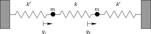 |
Let  and
and  be the displacements of the first and second masses,
respectively, from the equilibrium state. It follows that the
extensions of the left-hand, middle, and right-hand springs are
,
be the displacements of the first and second masses,
respectively, from the equilibrium state. It follows that the
extensions of the left-hand, middle, and right-hand springs are
,  , and
, and  , respectively. The kinetic energy of the system takes the
form
, respectively. The kinetic energy of the system takes the
form
 |
(819) |
whereas the potential energy is written
![\begin{displaymath}
U= \frac{1}{2}\left[k'\,q_1^{\,2} + k\,(q_2-q_1)^2+ k'\,q_2^{\,2}\right].
\end{displaymath}](img1989.png) |
(820) |
The above expression can be rearranged to give
![\begin{displaymath}
U= \frac{1}{2}\left[(k+k')\,q_1^{\,2} -2\,k\,q_1\,q_2 + (k+k')\,q_2^{\,2}\right].
\end{displaymath}](img1990.png) |
(821) |
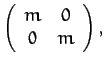
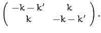
A comparison of Equations (819) and (821) with the standard
forms (775) and (780) yields the following
expressions for the mass matrix,  , and the force matrix,
  :
:
Now, the equation of motion of the system takes the form [see Equation (786)]
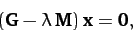 |
(824) |
where  is the column vector of the and values.
The solubility condition for the above equation is
is the column vector of the and values.
The solubility condition for the above equation is
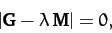 |
(825) |
or
![\begin{displaymath}
\left\vert\begin{array}{cc}
-k-k'-\lambda\,m& k\\ [0.5ex]
k&-k-k'-\lambda\,m
\end{array}\right\vert = 0,
\end{displaymath}](img1997.png) |
(826) |
which yields the following quadratic equation for the eigenvalue  :
:
 |
(827) |
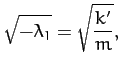
The two roots of the above equation are
The fact that the roots are negative implies that both normal modes are
oscillatory in nature: i.e., the original equilibrium is stable.
The characteristic oscillation frequencies of the modes are
Now, the first row of Equation (824) gives
 |
(832) |
Moreover, Equations (799) and (822) yield the following
normalization condition for the eigenvectors:
 |
(833) |
for  . It follows that the two eigenvectors are
According to Equations (830)-(831) and (834)-(835), our two degree of freedom system possesses two normal modes. The first mode oscillates at the frequency  , and is a purely symmetric
mode: i.e.,
, and is a purely symmetric
mode: i.e.,  . Note that such a mode does not stretch
the middle spring. Hence, is independent of . In fact, is simply the characteristic oscillation frequency of a mass on the end of a spring of spring constant . The second mode
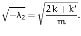
oscillates at the frequency
. Note that such a mode does not stretch
the middle spring. Hence, is independent of . In fact, is simply the characteristic oscillation frequency of a mass on the end of a spring of spring constant . The second mode
oscillates at the frequency  , and is a purely
anti-symmetric mode: i.e.,
, and is a purely
anti-symmetric mode: i.e.,  . Since such a mode
stretches the middle spring, the second mode experiences a greater restoring force than the first, and hence has a higher oscillation frequency: i.e.,
. Since such a mode
stretches the middle spring, the second mode experiences a greater restoring force than the first, and hence has a higher oscillation frequency: i.e.,
 .
.
Note, finally, from Equations (809) and (822), that the normal
coordinates of the system are:
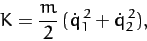
When expressed in terms of these normal coordinates, the kinetic
and potential energies of the system reduce to
respectively.
Next: Triatomic Molecule
Up: Coupled Oscillations
Previous: Normal Coordinates
Richard Fitzpatrick
2011-03-31