


Next: Conic Sections
Up: Planetary Motion
Previous: Conservation Laws
Polar Coordinates
We can determine the instantaneous position of our planet in the
 -
- plane in terms of standard Cartesian coordinates, (, ),
or polar coordinates, (
plane in terms of standard Cartesian coordinates, (, ),
or polar coordinates, ( ,
,  ), as illustrated in Figure 13. Here,
 and
and
 .
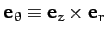
It is helpful to define two unit vectors,
.
It is helpful to define two unit vectors,
 and
and
 , at the
instantaneous position of the planet. The first always points radially away from the origin,
whereas the second is normal to the first, in the direction of increasing . As is easily demonstrated, the Cartesian components of
, at the
instantaneous position of the planet. The first always points radially away from the origin,
whereas the second is normal to the first, in the direction of increasing . As is easily demonstrated, the Cartesian components of
 and
and
 are
are
respectively.
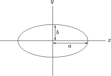
Figure 14:
An ellipse.
 |
We can write the position vector of our planet as
 |
(220) |
Thus, the planet's velocity becomes
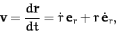 |
(221) |
where  is shorthand for
  . Note that
has a non-zero time-derivative (unlike a Cartesian unit vector) because its
direction changes as the planet moves around. As is easily demonstrated,
from differentiating Equation (218) with respect to time,
. Note that
has a non-zero time-derivative (unlike a Cartesian unit vector) because its
direction changes as the planet moves around. As is easily demonstrated,
from differentiating Equation (218) with respect to time,
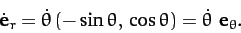 |
(222) |
Thus,
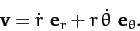 |
(223) |
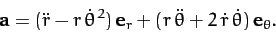
Now, the planet's acceleration is written
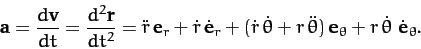 |
(224) |
Again,
has a non-zero time-derivative because its
direction changes as the planet moves around.
Differentiation of Equation (219) with respect to time yields
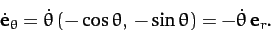 |
(225) |
Hence,
 |
(226) |
It follows that the equation of motion of our planet, (212), can be written
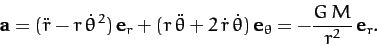 |
(227) |
Since and
are mutually orthogonal, we can separately equate the coefficients of both, in the above equation, to give
a radial equation of motion,
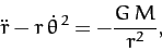 |
(228) |
and a tangential equation of motion,
 |
(229) |
Next: Conic Sections
Up: Planetary Motion
Previous: Conservation Laws
Richard Fitzpatrick
2011-03-31