Stability Equations

It is evident that if our system is initialized in some equilibrium state, with all of the $\dot{q}_i$ set to zero, then it will remain in this state for ever. But what happens if the system is slightly perturbed from the equilibrium state?

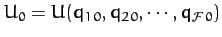
Let

$$q_i = q_{i\,0} + \delta q_i,$$ (774)

for $i=1,{\cal F}$, where the $\delta q_i$ are small. To lowest order in $\delta q_i$, the kinetic energy (770) can be written

$$K \simeq \frac{1}{2}\sum_{i,j=1,{\cal F}} M_{ij}\,\delta\dot{q}_i\,\delta\dot{q}_j,$$ (775)

where

$$M_{ij} = m_{ij}(q_{1\,0},q_{2\,0},\cdots,q_{{\cal F}\,0}),$$ (776)

and

$$M_{ij} = M_{ji}.$$ (777)

Note that the weights $M_{ij}$ in the quadratic form (775) are now constants.

Taylor expanding the potential energy function about the equilibrium state, up to second-order in the $\delta q_i$, we obtain

$$U \simeq U_0 - \sum_{i=1,{\cal F}} Q_{i\,0}\,\delta q_i - \frac{1}{2}\sum_{i,j=1,{\cal F}} G_{ij}\,\delta q_i \,\delta q_j,$$ (778)

where $U_0=U(q_{1\,0},q_{2\,0},\cdots, q_{{\cal F}\,0})$, the $Q_{i\,0}$ are specified in Equation (773), and

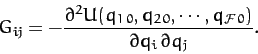$$G_{ij} = -\frac{\partial^2 U(q_{1\,0},q_{2\,0},\cdots, q_{{\cal F}\,0})}{\partial q_i\,\partial q_j}.$$ (779)

Now, we can set $U_0$ to zero without loss of generality. Moreover, according to Equation (773), the $Q_{i\,0}$ are all zero. Hence, the expression (778) reduces to

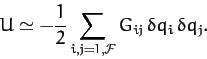$$U \simeq - \frac{1}{2}\sum_{i,j=1,{\cal F}} G_{ij}\,\delta q_i \,\delta q_j.$$ (780)

Note that, since 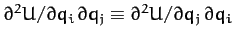$\partial^2 U/\partial q_i\,\partial q_j\equiv \partial^2 U/\partial q_j\,\partial q_i$, the constants weights $G_{ij}$ in the above quadratic form are invariant under interchange of the indices $i$ and $j$: i.e.,

$$G_{ij} = G_{ji}.$$ (781)

With $K$ and $U$ specified by the quadratic forms (775) and (780), respectively, Lagrange's equations of motion (772) reduce to

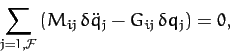$$\sum_{j=1,{\cal F}}\left(M_{ij}\,\delta\ddot{q}_j - G_{ij}\,\delta q_j\right) = 0,$$ (782)

for $i=1,{\cal F}$. Note that the above coupled differential equations are linear in the $\delta q_i$. It follows that the solutions are superposable. Let us search for solutions of the above equations in which all of the perturbed coordinates $\delta q_i$ have a common time variation of the form

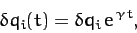$$\delta q_i(t) = \delta q_i\,{\rm e}^{\,\gamma\,t},$$ (783)

for $i=1,{\cal F}$. Now, Equations (782) are a set of ${\cal F}$ second-order differential equations. Hence, the most general solution contains $2{\cal F}$ arbitrary constants of integration. Thus, if we can find sufficient independent solutions of the form (783) to Equations (782) that the superposition of these solutions contains $2{\cal F}$ arbitrary constants then we can be sure that we have found the most general solution. Equations (782) and (783) yield

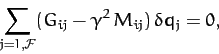$$\sum_{j=1,{\cal F}}(G_{ij}- \gamma^2\,M_{ij})\,\delta q_j = 0,$$ (784)

which can be written more succinctly as a matrix equation:

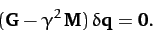$$({\bf G} - \gamma^2\,{\bf M})\,\delta\bf {q} = {\bf0}.$$ (785)

Here, ${\bf G}$ is the real [see Equation (779)] symmetric [see Equation (781)] ${\cal F}\times {\cal F}$ matrix of the $G_{ij}$ values. Furthermore, ${\bf M}$ is the real [see Equation (770)] symmetric [see Equation (777)] ${\cal F}\times {\cal F}$ matrix of the $M_{ij}$ values. Finally, $\delta {\bf q}$ is the $1\times {\cal F}$ vector of the $\delta q_i$ values, and ${\bf0}$ is a null vector.