Next: Exercises
Up: Hamiltonian Dynamics
Previous: Constrained Lagrangian Dynamics
Consider a dynamical system with  degrees of freedom which is described
by the generalized coordinates
degrees of freedom which is described
by the generalized coordinates  , for
, for  . Suppose that
neither the kinetic energy,
. Suppose that
neither the kinetic energy,  , nor the potential energy,
  , depend
explicitly on the time,
, depend
explicitly on the time,  . Now, in conventional dynamical systems, the potential energy is generally independent of the
  , whereas the kinetic
energy takes the form of a homogeneous quadratic function of
the . In other words,
, whereas the kinetic
energy takes the form of a homogeneous quadratic function of
the . In other words,
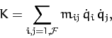 |
(744) |
where the  depend on the , but not on the .
It is easily demonstrated from the above equation that
depend on the , but not on the .
It is easily demonstrated from the above equation that
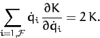 |
(745) |
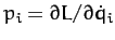
Recall, from Section 9.8, that generalized momentum conjugate to the  th
generalized coordinate is defined
th
generalized coordinate is defined
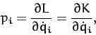 |
(746) |
where  is the Lagrangian of the system, and we have made use of the fact that is independent of the . Consider the
function
is the Lagrangian of the system, and we have made use of the fact that is independent of the . Consider the
function
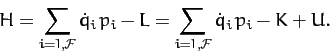 |
(747) |
If all of the conditions discussed above are satisfied then Equations (745)
and (746)
yield
 |
(748) |
In other words, the function  is equal to the total energy of the system.
Consider the variation of the function . We have
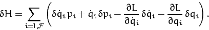 |
(749) |
The first and third terms in the bracket cancel, because
 . Furthermore, since Lagrange's equation
can be written
. Furthermore, since Lagrange's equation
can be written
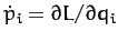 (see Section 9.8), we obtain
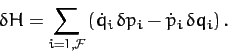 |
(750) |
Suppose, now, that we can express the total energy of the system, , solely
as a function of the and the  , with no explicit
dependence on the . In other words, suppose that we
can write
, with no explicit
dependence on the . In other words, suppose that we
can write  . When the energy is written
in this fashion it is generally termed the Hamiltonian of the system. The variation of the Hamiltonian function takes the form
. When the energy is written
in this fashion it is generally termed the Hamiltonian of the system. The variation of the Hamiltonian function takes the form
 |
(751) |
A comparison of the previous two equations yields
for . These  first-order differential equations are known
as Hamilton's equations. Hamilton's equations are often a
useful alternative to Lagrange's equations, which take the
form of second-order differential equations.
first-order differential equations are known
as Hamilton's equations. Hamilton's equations are often a
useful alternative to Lagrange's equations, which take the
form of second-order differential equations.
Consider a one-dimensional harmonic oscillator. The kinetic and potential
energies of the system are written
 and
and
 , where
  is the displacement,
  the mass, and
  .
The generalized momentum conjugate to is
.
The generalized momentum conjugate to is
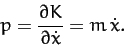 |
(754) |
Hence, we can write
 |
(755) |
So, the Hamiltonian of the system takes the form
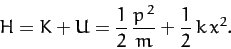 |
(756) |
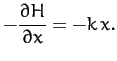
Thus, Hamilton's equations, (752) and (753), yield
Of course, the first equation is just a restatement of Equation (754), whereas the second is Newton's second law of motion for the
system.
Consider a particle of mass moving in the central potential  .
In this case,
.
In this case,
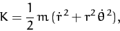 |
(759) |
where  are polar coordinates. The generalized momenta conjugate to
  and
and  are
are
respectively.
Hence, we can write
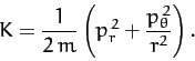 |
(762) |
Thus, the Hamiltonian of the system takes the form
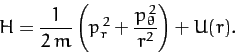 |
(763) |
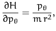
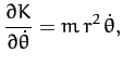
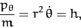
In this case, Hamilton's equations yield
which are just restatements of Equations (760) and (761), respectively,
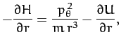
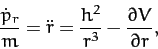
as well as
The last equation implies that
 |
(768) |
where  is a constant. This can be combined with Equation (766)
to give
is a constant. This can be combined with Equation (766)
to give
 |
(769) |
where  . Of course, Equations (768) and (769) are the
conventional equations of motion for a particle moving in a central potential--see Chapter 5.
. Of course, Equations (768) and (769) are the
conventional equations of motion for a particle moving in a central potential--see Chapter 5.
Next: Exercises
Up: Hamiltonian Dynamics
Previous: Constrained Lagrangian Dynamics
Richard Fitzpatrick
2011-03-31