


Next: Conditional Variation
Up: Hamiltonian Dynamics
Previous: Introduction
Calculus of Variations
It is a well-known fact, first enunciated by Archimedes, that the shortest
distance between two points in a plane is a straight-line. However, suppose that
we wish to demonstrate this result from first principles. Let us consider the
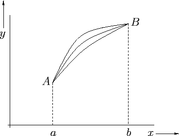
length,  , of various curves,
  , which run between two fixed
points,
, which run between two fixed
points,  and
and  , in a plane, as illustrated in Figure 35. Now, takes the form
![\begin{displaymath}
l = \int_A^B [dx^2 + dy^2]^{1/2} = \int_a^b [1 + y'^{\,2}(x)]^{1/2}\,dx,
\end{displaymath}](img1717.png) |
(675) |
where
 . Note that is a function of the function .
In mathematics, a function of a function is termed a functional.
. Note that is a function of the function .
In mathematics, a function of a function is termed a functional.
Figure 35:
Different paths between points and .
 |
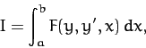
Now, in order to find the shortest path between points and , we need to minimize the functional with respect to small variations
in the function , subject to the constraint that the end points,
and , remain fixed. In other words, we need to solve
 |
(676) |
The meaning of the above equation is that if
 , where
  is small, then the first-order variation in ,
denoted
is small, then the first-order variation in ,
denoted  ,
vanishes. In other words,
,
vanishes. In other words,
 . The particular function
for which
. The particular function
for which  obviously yields an extremum of (i.e., either a maximum or a minimum). Hopefully,
in the case under consideration,
it yields a minimum of .
obviously yields an extremum of (i.e., either a maximum or a minimum). Hopefully,
in the case under consideration,
it yields a minimum of .
Consider a general functional of the form
 |
(677) |
where the end points of the integration are fixed.
Suppose that
. The first-order variation in  is written
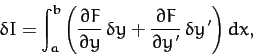 |
(678) |
where
 . Setting
  to zero, we
obtain
to zero, we
obtain
 |
(679) |
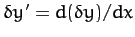
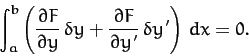
This equation must be satisfied for all possible small perturbations .
Integrating the second term in the integrand of the above equation by
parts, we get
![\begin{displaymath}
\int_a^b\left[\frac{\partial F}{\partial y}- \frac{d}{dx}\!\...
... +\left[\frac{\partial F}{\partial y'}\,\delta y\right]_a^b=0.
\end{displaymath}](img1731.png) |
(680) |
Now, if the end points are fixed then  at
at
 and
and  . Hence, the last term on the left-hand side of the
above equation is zero. Thus, we obtain
. Hence, the last term on the left-hand side of the
above equation is zero. Thus, we obtain
![\begin{displaymath}
\int_a^b\left[\frac{\partial F}{\partial y}- \frac{d}{dx}\!\left(\frac{\partial F}{\partial y'}\right)\right]\delta y\,dx =0.
\end{displaymath}](img1734.png) |
(681) |
The above equation must be satisfied for all small perturbations
. The only way in which this is possible is for the
expression enclosed in square brackets in the integral to be zero. Hence, the functional
attains an extremum value whenever
 |
(682) |
This condition is known as the Euler-Lagrange equation.
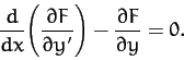
Let us consider some special cases. Suppose that  does not explicitly
depend on
does not explicitly
depend on  . It follows that
 . Hence,
the Euler-Lagrange equation (682) simplifies to
. Hence,
the Euler-Lagrange equation (682) simplifies to
 |
(683) |
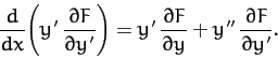
Next, suppose that does not depend explicitly on  . Multiplying
Equation (682) by
. Multiplying
Equation (682) by  , we obtain
 |
(684) |
However,
 |
(685) |
Thus, we get
 |
(686) |
Now, if is not an explicit function of then the right-hand side of
the above equation is the total derivative of , namely  .
Hence, we obtain
.
Hence, we obtain
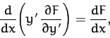 |
(687) |
which yields
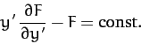 |
(688) |
Returning to the case under consideration, we have
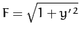 , according to Equation (675) and (677). Hence, is not
an explicit function of , so Equation (683) yields
, according to Equation (675) and (677). Hence, is not
an explicit function of , so Equation (683) yields
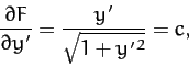 |
(689) |
where  is a constant. So,
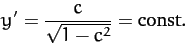 |
(690) |
Of course,
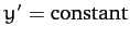 is the equation of a straight-line. Thus, the shortest distance between two fixed points in a plane is indeed a
straight-line.
is the equation of a straight-line. Thus, the shortest distance between two fixed points in a plane is indeed a
straight-line.
Next: Conditional Variation
Up: Hamiltonian Dynamics
Previous: Introduction
Richard Fitzpatrick
2011-03-31