Next: Atwood Machines
Up: Lagrangian Dynamics
Previous: Lagrange's Equation
Motion in a Central Potential
Consider a particle of mass  moving in two dimensions in the central potential
  . This is clearly a two degree of freedom dynamical system.
As described in Section 5.5, the particle's instantaneous position
is most conveniently specified in terms of the plane polar
coordinates
. This is clearly a two degree of freedom dynamical system.
As described in Section 5.5, the particle's instantaneous position
is most conveniently specified in terms of the plane polar
coordinates  and
and  . These are our two generalized coordinates.
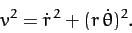
According to Equation (223), the square of the particle's velocity
can be written
. These are our two generalized coordinates.
According to Equation (223), the square of the particle's velocity
can be written
 |
(614) |
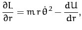
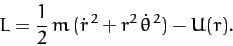
Hence, the Lagrangian of the system takes the form
 |
(615) |
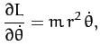
Note that
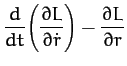
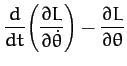
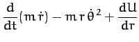
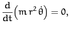
Now, Lagrange's equation (613) yields the equations of motion,
Hence, we obtain
or
where  , and
, and  is a constant. We recognize Equations (622) and (623) as the equations
we derived in Chapter 5 for motion in a central potential.
The advantage of the Lagrangian method of deriving these equations is
that we avoid having to express the acceleration in terms of the generalized
coordinates and .
is a constant. We recognize Equations (622) and (623) as the equations
we derived in Chapter 5 for motion in a central potential.
The advantage of the Lagrangian method of deriving these equations is
that we avoid having to express the acceleration in terms of the generalized
coordinates and .
Next: Atwood Machines
Up: Lagrangian Dynamics
Previous: Lagrange's Equation
Richard Fitzpatrick
2011-03-31