Next: Motion in a General
Up: Planetary Motion
Previous: Orbital Energies
In a nutshell, the so-called Kepler problem consists of determining
the radial and angular coordinates,  and
and  , respectively, of
an object in a Keplerian orbit about the Sun as a function of time.
, respectively, of
an object in a Keplerian orbit about the Sun as a function of time.
Consider an object in a general Keplerian orbit about the Sun which
passes through its perihelion point,  and
and  , at
, at  . It
follows from the previous analysis that
. It
follows from the previous analysis that
 |
(276) |
and
 |
(277) |
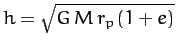
where  ,
,
 , and
, and
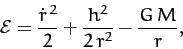
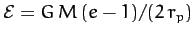 are the orbital eccentricity, angular momentum per unit mass, and
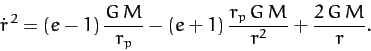
energy per unit mass, respectively. The above equation can be rearranged to
give
are the orbital eccentricity, angular momentum per unit mass, and
energy per unit mass, respectively. The above equation can be rearranged to
give
 |
(278) |
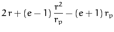
Taking the square-root, and integrating, we obtain
![\begin{displaymath}
\int_{r_p}^r\frac{r\,dr}{[2\,r + (e-1)\,r^2/r_p - (e+1)\,r_p]^{1/2}} =
\sqrt{G\,M}\,\,t.
\end{displaymath}](img795.png) |
(279) |
Consider an elliptical orbit characterized by  . Let us write
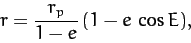 |
(280) |
where  is termed the elliptic anomaly. In fact, is an angle which
varies between
is termed the elliptic anomaly. In fact, is an angle which
varies between  and
and  . Moreover, the perihelion point corresponds to
 , and the aphelion point to
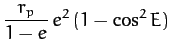
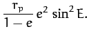
  . Now,
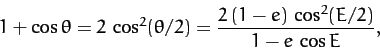
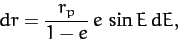 |
(281) |
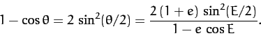
whereas
Thus, Equation (279) reduces to
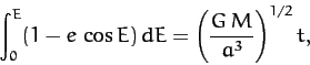 |
(283) |
where 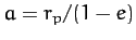 . This equation can immediately be integrated to give
 |
(284) |
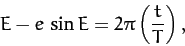
where
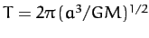 is the orbital period. Equation (284),
which is known as Kepler's equation, is a transcendental equation
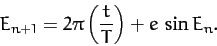
which does not possess a simple analytic solution. Fortunately, it is fairly straightforward to
solve numerically. For instance, using an iterative approach,
if
is the orbital period. Equation (284),
which is known as Kepler's equation, is a transcendental equation
which does not possess a simple analytic solution. Fortunately, it is fairly straightforward to
solve numerically. For instance, using an iterative approach,
if  is the
  th guess then
 |
(285) |
The above iteration scheme converges very rapidly (except in the limit
as
 ).
).
Equations (276) and (280) can be combined
to give
 |
(286) |
Thus,
 |
(287) |
and
 |
(288) |
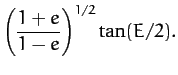
The previous two equations imply that
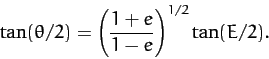 |
(289) |
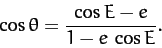
We conclude that, in the case of an elliptical orbit, the solution of the Kepler problem reduces to the solution of the following three equations:
Here,
and . Incidentally, it is clear that if
 then
then
 , and
, and
 . In other words, the motion is periodic with period
 .
.
For the case of a parabolic orbit, characterized by  , similar analysis to
the above yields:
, similar analysis to
the above yields:
Here,  is termed the parabolic anomaly, and varies between
 and
and  , with the perihelion point corresponding to
  . Note that Equation (293) is a cubic equation,
possessing a single real root,
which can, in principle, be solved analytically. However, a numerical
solution is generally more convenient.
. Note that Equation (293) is a cubic equation,
possessing a single real root,
which can, in principle, be solved analytically. However, a numerical
solution is generally more convenient.
Finally, for the case of a hyperbolic orbit, characterized by  ,
we obtain:
,
we obtain:
Here,  is termed the hyperbolic anomaly, and varies between
and , with the perihelion point corresponding to
is termed the hyperbolic anomaly, and varies between
and , with the perihelion point corresponding to  . Moreover,
  . As in the elliptical
case, Equation (296) is a transcendental equation which is most easily solved numerically.
. As in the elliptical
case, Equation (296) is a transcendental equation which is most easily solved numerically.
Next: Motion in a General
Up: Planetary Motion
Previous: Orbital Energies
Richard Fitzpatrick
2011-03-31