![$\displaystyle \int_0^\infty\left[\frac{a_1^{\,2}\,a_2^{\,2}}{(a_1^{\,2}+u)\,(a_2^{\,2}+u)}- \frac{a_3^{\,2}}{(a_3^{\,2}+u)}\right]\frac{du}{\mit\Delta} = 0.$](img924.png) |
(2.133) |
| (2.134) | ||
| (2.135) |
| (2.136) | ||
| (2.137) |
| (2.138) |
Let
![]() . Here,
. Here, ![]() corresponds to
corresponds to
![]() , and
, and
![]() to
to ![]() . Equations (2.115) and (2.114) transform to (Darwin 1886)
. Equations (2.115) and (2.114) transform to (Darwin 1886)
 |
(2.143) |
The constraint (2.139) is obviously satisfied in the limit
![]() , because this implies
that
, because this implies
that
![]() and
and
![]() ,
,
![]() . Of course, this limit corresponds to the axisymmetric Maclaurin spheroids discussed in the previous section. Carl Jacobi (1804-1851), in 1834, was the first researcher to obtain the
very surprising result that Equation (2.139) also has non-axisymmetric ellipsoidal solutions characterized by
. Of course, this limit corresponds to the axisymmetric Maclaurin spheroids discussed in the previous section. Carl Jacobi (1804-1851), in 1834, was the first researcher to obtain the
very surprising result that Equation (2.139) also has non-axisymmetric ellipsoidal solutions characterized by
![]() . These solutions are known as the Jacobi ellipsoids
in his honor. The properties of the Jacobi ellipsoids, as determined from Equations (2.139), (2.140), (2.144), and (2.145),
are set out in Table 2.2, and illustrated in Figures 2.5 and 2.6. It can be seen that the
sequence of Jacobi ellipsoids bifurcates from the sequence of Maclaurin spheroids when
. These solutions are known as the Jacobi ellipsoids
in his honor. The properties of the Jacobi ellipsoids, as determined from Equations (2.139), (2.140), (2.144), and (2.145),
are set out in Table 2.2, and illustrated in Figures 2.5 and 2.6. It can be seen that the
sequence of Jacobi ellipsoids bifurcates from the sequence of Maclaurin spheroids when
![]() . Moreover, there are no Jacobi ellipsoids
with
. Moreover, there are no Jacobi ellipsoids
with
![]() .
However, as
.
However, as ![]() increases above
this critical value, the eccentricity,
increases above
this critical value, the eccentricity, ![]() , of the Jacobi ellipsoids in the
, of the Jacobi ellipsoids in the ![]() -
-![]() plane grows rapidly, approaching unity as
plane grows rapidly, approaching unity as
![]() approaches unity. Thus, in the limit
approaches unity. Thus, in the limit
![]() , in which a Maclaurin spheroid collapses to a disk in the
, in which a Maclaurin spheroid collapses to a disk in the ![]() -
-![]() plane, a Jacobi ellipsoid collapses to a line running along the
plane, a Jacobi ellipsoid collapses to a line running along the ![]() -axis.
Note, from Figures 2.5 and 2.6, that, at fixed
-axis.
Note, from Figures 2.5 and 2.6, that, at fixed ![]() , the Jacobi ellipsoids have lower
angular velocity and angular momentum than Maclaurin spheroids (with the same mass and volume).
Furthermore, as is the case for a Maclaurin spheroid, there is a maximum angular velocity that a Jacobi ellipsoid can
have (i.e.,
, the Jacobi ellipsoids have lower
angular velocity and angular momentum than Maclaurin spheroids (with the same mass and volume).
Furthermore, as is the case for a Maclaurin spheroid, there is a maximum angular velocity that a Jacobi ellipsoid can
have (i.e.,
![]() ), but no maximum angular momentum.
), but no maximum angular momentum.
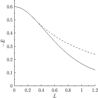 |
Figure 2.7 shows the mechanical energy of the Maclaurin spheroids and Jacobi ellipsoids plotted as a function of their
angular momentum. It can be seen that the Jacobi ellipsoid with a given angular momentum has a lower
energy that the corresponding Maclaurin spheroid (i.e., the spheroid with the same angular momentum, mass, and volume).
This is significant because, in the presence of a small amount of dissipation (i.e., viscosity), we would generally expect an isolated fluid system to slowly evolve toward the equilibrium
state with the lowest energy, subject to any global constraints on the system. For the case of a weakly viscous, isolated, rotating,
liquid planet, the relevant constraints are that the mass, volume, and net angular momentum of the system cannot spontaneously change. Thus, we expect such a planet to evolve toward the equilibrium state with the lowest energy for a given mass, volume, and angular momentum. This suggests, from
Figure 2.7, that at relatively high angular momentum (i.e.,
![]() ,
,
![]() ), when the Jacobi ellipsoid solutions exist, they are stable equilibrium states (because there
is no lower energy state to which the system can evolve), whereas the Maclaurin spheroids are unstable. On the other hand, at relatively low angular momentum (i.e.,
), when the Jacobi ellipsoid solutions exist, they are stable equilibrium states (because there
is no lower energy state to which the system can evolve), whereas the Maclaurin spheroids are unstable. On the other hand, at relatively low angular momentum (i.e.,
![]() ,
,
![]() ), when there
are no Jacobi ellipsoid solutions, the Maclaurin spheroids are stable equilibrium states (again, because there is no
lower energy state to which they can evolve). These predictions are borne out by the results of direct stability analysis performed on the Maclaurin
spheroids and Jacobi ellipsoids (Chandrasekhar 1969). In fact, such stability studies demonstrate that the Maclaurin spheroids are unstable in the
presence of weak dissipation for
), when there
are no Jacobi ellipsoid solutions, the Maclaurin spheroids are stable equilibrium states (again, because there is no
lower energy state to which they can evolve). These predictions are borne out by the results of direct stability analysis performed on the Maclaurin
spheroids and Jacobi ellipsoids (Chandrasekhar 1969). In fact, such stability studies demonstrate that the Maclaurin spheroids are unstable in the
presence of weak dissipation for
![]() , and unconditionally unstable for
, and unconditionally unstable for
![]() .
The Jacobi ellipsoids, on the other hand, are unconditionally stable for
.
The Jacobi ellipsoids, on the other hand, are unconditionally stable for
![]() , but are unconditionally
unstable for
, but are unconditionally
unstable for
![]() , evolving toward lower energy ``pear shaped'' equilibria (which are, themselves, unstable in the
presence of weak dissipation).
, evolving toward lower energy ``pear shaped'' equilibria (which are, themselves, unstable in the
presence of weak dissipation).
![$\displaystyle E(\gamma,\alpha)- 2\,F(\gamma,\alpha) +\left[\frac{1+(\sin\alpha\,\tan\beta\,\cos\gamma)^2}{\cos^2\alpha}\right] E(\gamma,\alpha)$](img940.png)
![$\displaystyle \widehat{\omega}^{\,2} =2\left[\frac{F(\gamma,\alpha)-E(\gamma,\a...
...n^3\gamma\,\cos^2\alpha}-\frac{\cos^2\beta}{\tan^2\gamma\,\cos^2\alpha}\right],$](img942.png)