


Next: Multi-Function Variation
Up: Calculus of Variations
Previous: Euler-Lagrange Equation
Suppose that we wish to find the function  which
maximizes or minimizes the functional
which
maximizes or minimizes the functional
 |
(E.17) |
subject to the constraint that the value of
 |
(E.18) |
remains constant. We can achieve our goal by finding an extremum of the new functional
 , where
 is an undetermined function. We know
that
is an undetermined function. We know
that
 , because the value of
  is fixed, so if
 then
then
 as well. In other words, finding an extremum of
  is equivalent
to finding an extremum of
is equivalent
to finding an extremum of  . Application of the Euler-Lagrange
equation yields
. Application of the Euler-Lagrange
equation yields
![$\displaystyle \frac{d}{dx}\!\left(\frac{\partial F}{\partial y'}\right)-\frac{\...
...da\,G]}{\partial y'}\right)-\frac{\partial [\lambda\,G]}{\partial y}\right]= 0.$](img7334.png) |
(E.19) |
In principle, the previous equation, together with the constraint (E.18),
yields the functions
and
. Incidentally,  is generally
termed a Lagrange multiplier. If
is generally
termed a Lagrange multiplier. If  and
and  have no explicit
  -dependence then
is usually a constant.
-dependence then
is usually a constant.
As an example, consider the following famous problem. Suppose that a uniform
chain of fixed length  is suspended by its ends from
two equal-height fixed points that are a distance
is suspended by its ends from
two equal-height fixed points that are a distance  apart, where
  .
What is the equilibrium configuration of the chain?
.
What is the equilibrium configuration of the chain?
Suppose that the chain has the uniform density per unit length  .
Let the
- and
.
Let the
- and  -axes be horizontal and vertical, respectively, and
let the two ends of the chain lie at
-axes be horizontal and vertical, respectively, and
let the two ends of the chain lie at
 . The equilibrium configuration of the chain is specified by the function
, for
. The equilibrium configuration of the chain is specified by the function
, for
 , where
is the vertical distance of the chain below its end points at horizontal
position
. Of course,
, where
is the vertical distance of the chain below its end points at horizontal
position
. Of course,
 .
.
According to standard Newtonian dynamics, the stable equilibrium
state of a conservative dynamical system is one that minimizes
the system's potential energy (Fitzpatrick 2012). Now, the potential energy of the chain
is written
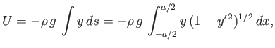 |
(E.20) |
where
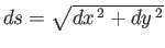 is an element of length along the chain, and
 is the acceleration due to gravity.
Hence, we need to minimize
is the acceleration due to gravity.
Hence, we need to minimize  with respect to small variations in
.
However, the variations in
must be such as to conserve the
fixed length of the chain. Hence, our minimization procedure is subject to
the constraint that
with respect to small variations in
.
However, the variations in
must be such as to conserve the
fixed length of the chain. Hence, our minimization procedure is subject to
the constraint that
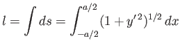 |
(E.21) |
remains constant.
It follows, from the previous discussion, that we need to minimize the
functional
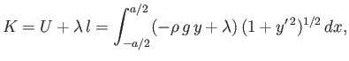 |
(E.22) |
where
is an, as yet, undetermined constant. Because the integrand
in the functional does not depend explicitly on
, we have
from Equation (E.14) that
 |
(E.23) |
where  is a constant. This expression reduces to
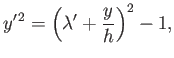 |
(E.24) |
where
 , and
, and
 .
.
Let
 |
(E.25) |
Making this substitution, Equation (E.24) yields
 |
(E.26) |
Hence,
 |
(E.27) |
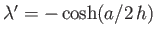
where  is a constant. It follows from Equation (E.25) that
![$\displaystyle y(x) =-h\,[\lambda' + \cosh(-x/h + c)].$](img7350.png) |
(E.28) |
The previous solution contains three undetermined constants,  ,
,  , and
. We can
eliminate two of these constants by application of the boundary
conditions
, and
. We can
eliminate two of these constants by application of the boundary
conditions
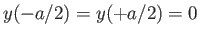
 . This yields
 |
(E.29) |
Hence,  , and
, and
 . It follows that
![$\displaystyle y(x) = h\,[\cosh(a/2\,h) - \cosh(x/h)].$](img7356.png) |
(E.30) |
The final unknown constant,
, is determined via the application of
the constraint (E.21). Thus,
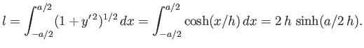 |
(E.31) |
Hence, the equilibrium configuration of the chain is given by the curve
(E.30), which is known as a catenary (from the Latin for chain), where the parameter
satisfies
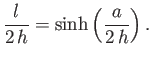 |
(E.32) |
Next: Multi-Function Variation
Up: Calculus of Variations
Previous: Euler-Lagrange Equation
Richard Fitzpatrick
2016-01-22