Next: Non-Global Ocean Tides
Up: Terrestrial Ocean Tides
Previous: Response to Equilibrium Harmonic
Suppose that the surface of the Earth is completely covered by an ocean of uniform mean depth  .
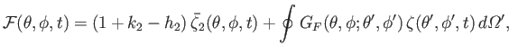
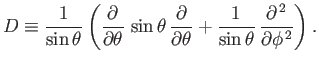
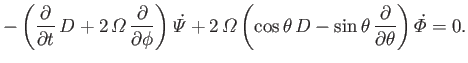
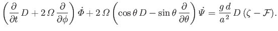
The motion of this ocean under the action of the tide generating potential is governed by
the Laplace tidal equations, (12.139)-(12.141), which can be written
.
The motion of this ocean under the action of the tide generating potential is governed by
the Laplace tidal equations, (12.139)-(12.141), which can be written
where
 |
(12.152) |
and
Here,
 .
.
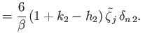
It is convenient to write (Love 1913)
It follows from Equation (12.153) that
 |
(12.157) |
where
 |
(12.158) |
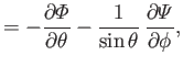
Forming
![% latex2html id marker 87749
$ (\sin\theta)^{-1}\,\partial(\ref{e129c})/\partial\phi-(\sin\theta)^{-1}\,\partial[\sin\theta(\ref{e130c})/\partial\theta]$](img4665.png) , we
obtain
, we
obtain
 |
(12.159) |
Similarly, forming
![% latex2html id marker 87753
$ -(\sin\theta)^{-1}\,(\partial/\partial\theta)\,[\sin\theta\,(\ref{e129c})]
-(\sin\theta)^{-1}\,\partial(\ref{e130c})/\partial\phi$](img4667.png) , we get
, we get
 |
(12.160) |
Let
 . Consider the response,
 , of the ocean to a particular harmonic of the forcing term that takes the form [see Equation (12.143)]
 |
(12.161) |
where
 is a constant. We can write
where the
 are associated Legendre functions, and the
  and
and
 are constants.
Now, by definition (Abramowitz and Stegun 1965),
are constants.
Now, by definition (Abramowitz and Stegun 1965),
 |
(12.164) |
Hence, Equations (12.161) and (12.166) give
 |
(12.165) |
Equations (12.136) and (12.138) imply that
 |
(12.166) |
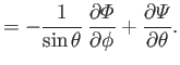
It follows from Equations (12.163) and (12.164) that
![$\displaystyle \sum_{n=1,\infty}\left\{{\mit\Psi}_n\left[-f_j\,n\,(n+1)+m_j\righ...
...ac{(1-\mu^{\,2})}{n\,(n+1)}\,\frac{d}{d\mu}\right]P_n^{\,m_j}(\mu)\right\} = 0,$](img4681.png) |
(12.167) |
and
where (Lamb 1993)
However, as is well known (Abramowitz and Stegun 1965),
Equations (12.171), (12.172), (12.175), and (12.176) can be combined to give
![$\displaystyle \left[m_j-n\,(n+1)\,f_j\right]{\mit\Psi}_n + \left(\frac{n+1}{n}\...
...n-1}\right)z_{n-1}+\left(\frac{n}{n+1}\,\frac{n+m_j+1}{2\,n+3}\right)z_{n+1}=0,$](img4690.png) |
(12.172) |
and
Finally, Equations (12.177) and (12.178) yield the tridiagonal matrix equation (Love 1913)
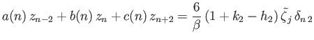 |
(12.174) |
for  ,
,  ,
,  ,
,  , where
 |
![$\displaystyle = - \frac{f_j\,n\,(n+1)\,(n-m_j-1)\,(n-m_j)}{(2\,n-3)\,(2\,n-1)\,[m_j-n\,(n-1)\,f_j]},$](img4698.png) |
(12.175) |
 |
![$\displaystyle = \frac{n\,(n+1)}{\beta}\left(1-[1+k_n'-h_n']\,\alpha_n\right) + \frac{m_j\,f_j}{n\,(n+1)}-f_j^{\,2}$](img4700.png) |
|
| |
![$\displaystyle \phantom{=}- \frac{f_j\,(n-1)^2\,(n+1)\,(n-m_j)\,(n+m_j)}{n\,(2\,n-1)\,(2\,n+1)\,[m_j-n\,(n-1)\,f_j]}$](img4701.png) |
|
| |
![$\displaystyle \phantom{=}-\frac{f_j\,(n+2)^2\,n\,(n-m_j+1)\,(n+m_j+1)}{(n+1)\,(2\,n+1)\,(2\,n+3)\,[m_j-(n+1)\,(n+2)\,f_j]},$](img4702.png) |
(12.176) |
 |
![$\displaystyle =-\frac{f_j\,n\,(n+1)\,(n+m_j+1)\,(n+m_j+2)}{(2\,n+3)\,(2\,n+5)\,[m_j-(n+1)\,(n+2)\,f_j]}.$](img4704.png) |
(12.177) |
Note that  .
The solution of a tridiagonal matrix equation is, of course, a relatively trivial numerical exercise (Press, et al. 2007).
.
The solution of a tridiagonal matrix equation is, of course, a relatively trivial numerical exercise (Press, et al. 2007).
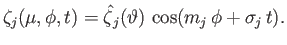
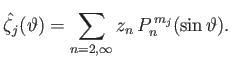
We can most conveniently characterize the  th tidal harmonic in terms of the function
 ,
which is defined such that
,
which is defined such that
 |
(12.178) |
Here,
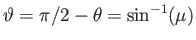 represents planetary latitude.
It follows that
represents planetary latitude.
It follows that
 |
(12.179) |
The
 ,
,  , and
, and  values for the various harmonics of the forcing term in the Laplace tidal equations for the Earth are specified in Table 12.3.
Note that, on the longitudinal meridian
values for the various harmonics of the forcing term in the Laplace tidal equations for the Earth are specified in Table 12.3.
Note that, on the longitudinal meridian  , the Moon and Sun culminate simultaneously at
  . Moreover, at this time, the Sun and Moon are both passing though the summer solstice, and the Moon is passing though its perigee.
The mean density of the Earth is such that
. Moreover, at this time, the Sun and Moon are both passing though the summer solstice, and the Moon is passing though its perigee.
The mean density of the Earth is such that
 (Yoder 1995).
Moreover, the mean depth of the Earth's oceans is
(Yoder 1995).
Moreover, the mean depth of the Earth's oceans is
 (Yoder 1995), which implies that
 .
Finally, the Earth responds
elastically to the relatively low-amplitude lunar and solar tidal gravitational fields in such a manner that
.
Finally, the Earth responds
elastically to the relatively low-amplitude lunar and solar tidal gravitational fields in such a manner that
 (Fitzpatrick 2012).
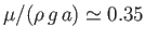
Figure:
Long-period solutions to the Laplace tidal equations (left panel) together with the corresponding equilibrium tides (right panel). The solid, dashed, and dash-dotted lines correspond to  ,
,  , and
, and  , respectively. Here,
 is measured in meters.
 |
Figures 12.1, 12.2, and 12.3 show the long-period, diurnal, and semi-diurnal solutions of the Laplace tidal
equations together with the corresponding equilibrium tides (i.e., the tides calculated in the absence of
ocean inertia),
![$\displaystyle \skew{5}\hat{\zeta}_j(\vartheta)= \left[\frac{1+k_2-h_2}{1-(1+k_2'-h_2')\,\alpha_2}\right]\skew{5}\tilde{\zeta}_j\,P_2^{\,m_j}(\sin\vartheta).$](img4716.png) |
(12.180) |
It can be seen from Figure 12.1 that the long-period solutions are direct (i.e., they have the same signs as the corresponding equilibrium tides).
However, the amplitudes of these solutions are about
times lower than those of the equilibrium tides. The
( ) and
(
) and
( ) solutions cause a slight increase in the equatorial bulge of the Earth's oceans when the Sun and Moon, respectively, pass through the equinoxes,
and a slight reduction when they pass through the solstices. The
(
) solutions cause a slight increase in the equatorial bulge of the Earth's oceans when the Sun and Moon, respectively, pass through the equinoxes,
and a slight reduction when they pass through the solstices. The
( ) solution causes a slight increase in the equatorial bulge of the Earth's oceans when the Moon
passes through its perigee, and a slight reduction when it passes through its apogee.
) solution causes a slight increase in the equatorial bulge of the Earth's oceans when the Moon
passes through its perigee, and a slight reduction when it passes through its apogee.
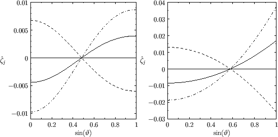
Figure:
Diurnal solutions to the Laplace tidal equations (left panel) together with the corresponding equilibrium tides (right panel). The solid, dashed, and dash-dotted lines correspond to  ,
,  , and
, and  , respectively. Here,
is measured in meters.
, respectively. Here,
is measured in meters.
 |
It can be seen from Figure 12.2 that the diurnal solutions are inverted (i.e., they have the opposite signs to the corresponding equilibrium tides).
The amplitude of
the
solution is about
times lower than that of the
equilibrium tide. The amplitudes of the
and
solutions are negligibly small. (In fact,
the amplitude of the
solution is identically zero.) The
( ) solution causes the Earth's oceans to displace slightly toward the Moon when it passes
through the equinoxes, and away from the Moon when it passes through the solstices.
) solution causes the Earth's oceans to displace slightly toward the Moon when it passes
through the equinoxes, and away from the Moon when it passes through the solstices.
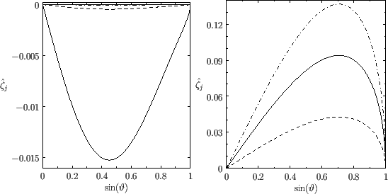
Figure:
Semi-diurnal solutions to the Laplace tidal equations (left panel) together with the corresponding equilibrium tides (right panel). The solid, dashed, and dash-dotted lines correspond to  ,
,  , and
, and  , respectively. Here,
is measured in meters.
, respectively. Here,
is measured in meters.
 |
Finally, it can be seen from Figure 12.3 that the semi-diurnal solutions are inverted in equatorial regions, and direct in polar regions. Moreover,
the amplitudes of these solutions are similar to those of the corresponding equilibrium tides. The dominant
( ) solution generates a high tide
at a particular point on the Earth's surface every
) solution generates a high tide
at a particular point on the Earth's surface every  hours. The
(
hours. The
( ) solution causes an enhancement of the high tide--a so-called spring tide--at the new and
full moons (i.e., every half a synodic month, or
) solution causes an enhancement of the high tide--a so-called spring tide--at the new and
full moons (i.e., every half a synodic month, or  days). Finally, the
(
days). Finally, the
( ) solution causes an enhancement of the spring tide--a so-called perigean spring tide--whenever the new or full moon coincides with the passage of the moon through its perigee.
The previously described global solutions to the Laplace tidal equations were first obtained (in simplified form) by Laplace (Lamb 1993). Let us consider how these solutions
compare with the observed terrestrial tides. One obvious prediction of the global solutions is that the time variation in ocean
depth at a given point on the Earth's surface should be expressible as a superposition of terms that oscillate at constant amplitude (but not
necessarily in phase with one another) with the periods specified in Table 12.3. This is indeed found to be the case (Cartwright 1999).
Another prediction is that the amplitudes of the long-period solutions should be small compared to the amplitudes
of the semi-diurnal solutions. This is also found to be the case. Yet another prediction is that amplitudes of the diurnal solutions should be small compared to the amplitudes
of the semi-diurnal solutions. This turns out not to be the case (Cartwright 1999). In fact, this predication is an artifact of the fact that we are assuming that
the ocean covering the Earth's surface is of constant mean depth. If we relax this assumption, and allow the ocean depth to vary in a realistic manner, then the amplitudes of the
semi-diurnal solutions become comparable to those of the diurnal solutions (Lamb 1993). The final prediction
is that a given solution is such that the tide at a given point on the Earth either oscillates in phase or in anti-phase with the corresponding
equilibrium solution (i.e., the tide is either direct or inverted). In particular, for the dominant
tide, this
implies that, at a given point on the Earth's surface, there should be either a tidal maximum or a tidal minimum whenever the Moon culminates.
It turns out that this is not the case (Cartwright 1999). Indeed, the observed phase difference between the
tide and the corresponding
equilibrium tide varies from place to place on the Earth's surface, and can take any value. In other words, high tide at a given point on the Earth can
occur three hours before the Moon culminates, or two hours after, et cetera, and the time lag between high tide and the culmination of the Moon
varies from place to place.
We conjecture that this effect is caused by the
continents impeding the flow of tidal waves around the Earth. Hence, we now need to consider tides in oceans that do not
cover the whole surface of the Earth.
Next: Non-Global Ocean Tides
Up: Terrestrial Ocean Tides
Previous: Response to Equilibrium Harmonic
Richard Fitzpatrick
2016-01-22


![$\displaystyle \frac{1}{\sin\theta}\left[\frac{\partial}{\partial\theta}\,(\sin\theta\,\xi)+ \frac{\partial\eta}{\partial\phi}\right] + \zeta$](img4651.png)
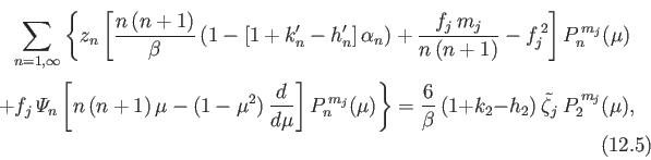


![$\displaystyle = -\left[\frac{n\,(n-m+1)}{2\,n+1}\right]P_{n+1}^{\,m}(\mu) + \left[\frac{(n+1)\,(n+m)}{2\,n+1}\right] P_{n-1}^{\,m}(\mu).$](img4689.png)
![$\displaystyle \left[\frac{n\,(n+1)}{\beta}\,(1-[1+k_n'-h_n']\,\alpha_n)+\frac{m_j\,f_j}{n\,(n+1)}-f_j^{\,2}\right]z_n$](img4691.png)
![$\displaystyle +f_j\left[\frac{(n-1)\,(n+1)\,(n-m_j)}{2\,n-1}\right]{\mit\Psi}_{n-1}$](img4692.png)
![$\displaystyle +f_j\left[\frac{n\,(n+2)\,(n+m_j+1)}{2\,n+3}\right]{\mit\Psi}_{n+1}$](img4693.png)