


Next: Wake Downstream of a
Up: Incompressible Boundary Layers
Previous: Self-Similar Boundary Layers
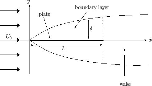
Boundary Layer on a Flat Plate
Consider a flat plate of length  , infinite width, and negligible thickness, that lies in the
  -
- plane, and whose
two edges correspond to
plane, and whose
two edges correspond to  and
and  . Suppose that the plate is immersed in a low viscosity fluid whose unperturbed velocity field is
 . (See Figure 8.4.) In the inviscid limit, the appropriate boundary condition at the
surface of the plate,
. (See Figure 8.4.) In the inviscid limit, the appropriate boundary condition at the
surface of the plate,  --corresponding to the requirement of zero normal velocity--is already satisfied by the unperturbed flow. Hence, the original flow is not modified
by the presence of the plate. However, when we take the finite viscosity of the fluid into account, an additional boundary
condition,
--corresponding to the requirement of zero normal velocity--is already satisfied by the unperturbed flow. Hence, the original flow is not modified
by the presence of the plate. However, when we take the finite viscosity of the fluid into account, an additional boundary
condition,  --corresponding to the no slip condition--must be satisfied at the plate. The
imposition of this additional constraint causes thin boundary layers, of thickness
--corresponding to the no slip condition--must be satisfied at the plate. The
imposition of this additional constraint causes thin boundary layers, of thickness
 , to form above and below the
plate. The fluid flow outside the boundary layers remains effectively inviscid, whereas that inside the
layers is modified by viscosity. It follows that the flow external to the layers is unaffected by the presence of the
plate. Hence, the tangential velocity at the outer edge of the boundary layers is
, to form above and below the
plate. The fluid flow outside the boundary layers remains effectively inviscid, whereas that inside the
layers is modified by viscosity. It follows that the flow external to the layers is unaffected by the presence of the
plate. Hence, the tangential velocity at the outer edge of the boundary layers is
 . This corresponds
to the case
. This corresponds
to the case  discussed in the previous section. [See Equation (8.52).] (Here, we are assuming that the flow upstream of the
trailing edge of the plate,
, is unaffected by the edge's presence, and, is, therefore, the same as if the plate were
of infinite length. Of course, the flow downstream of the edge is modified as a consequence of the finite length of the plate.)
discussed in the previous section. [See Equation (8.52).] (Here, we are assuming that the flow upstream of the
trailing edge of the plate,
, is unaffected by the edge's presence, and, is, therefore, the same as if the plate were
of infinite length. Of course, the flow downstream of the edge is modified as a consequence of the finite length of the plate.)
Figure 8.4:
Flow over a flat plate.
 |
Making use of the analysis contained in the previous section (with
), as well as the
fact that, by symmetry, the lower boundary layer is the mirror image of the upper one, the tangential velocity
profile across the both layers is written
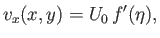 |
(8.64) |
where
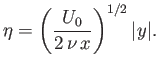 |
(8.65) |
Here,  is the solution of
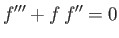 |
(8.66) |
that satisfies the boundary conditions
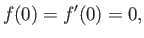 |
(8.67) |
and
Equation (8.66) is known as the Blasius equation.
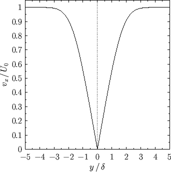
Figure:
Tangential velocity profile across the boundary layers located above and below a flat plate of negligible
thickness located at  .
.
 |
It is convenient to define the so-called displacement thickness of the upper boundary layer,
![$\displaystyle \delta(x) = \int_0^\infty \left[1-\frac{v_x(x,y)}{U_0}\right]dy,$](img2987.png) |
(8.70) |
which can be interpreted as the distance through which streamlines just outside the layer
are displaced laterally due to the retardation of the flow within the layer. (Of course, the thickness of the
lower boundary layer is the same as that of the upper layer.)
It follows that
![$\displaystyle \delta(x) = \left(\frac{\nu\,x}{U_0}\right)^{1/2}\sqrt{2}\int_0^\infty [1-f'(\eta)]\,d\eta.$](img2988.png) |
(8.71) |
In fact, the numerical solution of Equation (8.66), subject to the boundary conditions (8.67)-(8.69), yields
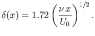 |
(8.72) |
Hence, the thickness of the boundary layer increases as the square root of the distance from the leading edge of the plate.
In particular, the thickness at the trailing edge of the plate is
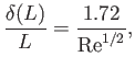 |
(8.73) |
where
 |
(8.74) |
is the appropriate Reynolds number for the interaction of the flow with the plate. Note that if
 then the
thickness of the boundary layer is much less than its length, as was previously assumed.
then the
thickness of the boundary layer is much less than its length, as was previously assumed.
The tangential velocity profile across the both boundary layers, which takes the form
![$\displaystyle v_x(x,y) = U_0\,f'\!\left[1.22\,\frac{\vert y\vert}{\delta(x)}\right],$](img2991.png) |
(8.75) |
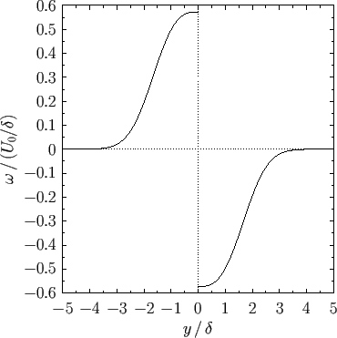
is plotted in Figure 8.5. In addition, the vorticity profile across the layers, which is
written
![$\displaystyle \omega(x,y) = - {\rm sgn}(y)\,1.22\,\frac{U_0}{\delta(x)}\,f''\!\left[1.22\,\frac{\vert y\vert}{\delta(x)}\right],$](img2992.png) |
(8.76) |
is shown in Figure 8.6. The vorticity is negative in the upper boundary layer (i.e.,  ), positive
in the lower boundary layer (i.e.,
), positive
in the lower boundary layer (i.e.,  ), and discontinuous across the plate (which is located at
).
Finally, the net viscous drag force per unit width (along the
-axis) acting on the plate in the
-direction is
), and discontinuous across the plate (which is located at
).
Finally, the net viscous drag force per unit width (along the
-axis) acting on the plate in the
-direction is
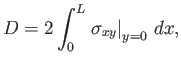 |
(8.77) |
where the factor of  is needed to take into account the presence of boundary layers both above and below the plate.
It follows from Equation (8.59) (with
) that
is needed to take into account the presence of boundary layers both above and below the plate.
It follows from Equation (8.59) (with
) that
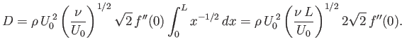 |
(8.78) |
In fact, the numerical solution of (8.66) yields
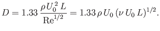 |
(8.79) |
Figure:
Vorticity profile across the boundary layers located above and below a flat plate of negligible
thickness located at
.
 |
The previous discussion is premised on the assumption that the flow in the upper (or lower) boundary layer is both steady and
-independent. It turns out that this assumption becomes invalid when the Reynolds number of the
layer,
 , exceeds a critical value which is about
  (Batchelor 2000). In this case, small-scale
-dependent disturbances spontaneously grow to large amplitude, and the
layer becomes turbulent. Because
(Batchelor 2000). In this case, small-scale
-dependent disturbances spontaneously grow to large amplitude, and the
layer becomes turbulent. Because
 , if the criterion for boundary layer turbulence is not
satisfied at the trailing edge of the plate,
, then it is not satisfied anywhere else in the layer. Thus, the
previous analysis, which neglects turbulence, remains valid provided
, if the criterion for boundary layer turbulence is not
satisfied at the trailing edge of the plate,
, then it is not satisfied anywhere else in the layer. Thus, the
previous analysis, which neglects turbulence, remains valid provided
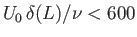 .
According to Equation (8.73), this implies that the analysis is valid when
.
According to Equation (8.73), this implies that the analysis is valid when
 , where
 is the Reynolds number of the external flow.
Figure 8.7:
Flow between two flat parallel plates.
 |
Consider, finally, the situation illustrated in Figure 8.7 in which an initially irrotational fluid
passes between two flat parallel plates. Let  be the perpendicular distance between the plates.
As we have seen, the finite viscosity of the fluid causes boundary layers to form on the inner surfaces of the upper and lower
plates. The flow within these layers possesses non-zero vorticity, and is significantly affected by viscosity. On the
other hand, the flow outside the layers is irrotational and essentially inviscid--this type of flow is usually
termed potential flow (because it can be derived from a velocity potential satisfying Laplace's equation).
The thickness of the two boundary layers increases like
be the perpendicular distance between the plates.
As we have seen, the finite viscosity of the fluid causes boundary layers to form on the inner surfaces of the upper and lower
plates. The flow within these layers possesses non-zero vorticity, and is significantly affected by viscosity. On the
other hand, the flow outside the layers is irrotational and essentially inviscid--this type of flow is usually
termed potential flow (because it can be derived from a velocity potential satisfying Laplace's equation).
The thickness of the two boundary layers increases like  , where
represents distance, parallel to the
flow, measured from the
leading edges of the plates. It follows that, as
increases, the region of potential flow shrinks in size, and
eventually disappears. (See Figure 8.7.) Assuming that, prior to merging, the two boundary layers do not significantly affect one another,
their thickness,
, where
represents distance, parallel to the
flow, measured from the
leading edges of the plates. It follows that, as
increases, the region of potential flow shrinks in size, and
eventually disappears. (See Figure 8.7.) Assuming that, prior to merging, the two boundary layers do not significantly affect one another,
their thickness,  , is given by formula (8.72), where
  is the speed of the incident fluid.
The region of potential flow thus extends from
(which corresponds to the leading edge of the plates) to
is the speed of the incident fluid.
The region of potential flow thus extends from
(which corresponds to the leading edge of the plates) to  , where
 |
(8.80) |
It follows that
 |
(8.81) |
where
 |
(8.82) |
Thus, when an irrotational high Reynolds number fluid passes between two parallel plates then the region of potential flow extends a comparatively long distance between the plates, relative to their spacing (i.e.,  ). By analogy, if an irrotational high Reynolds number fluid
passes into a pipe then the fluid remains essentially irrotational until it has travelled a considerable distance along the
pipe, compared to its diameter. Obviously, these conclusions are modified if the flow becomes turbulent.
). By analogy, if an irrotational high Reynolds number fluid
passes into a pipe then the fluid remains essentially irrotational until it has travelled a considerable distance along the
pipe, compared to its diameter. Obviously, these conclusions are modified if the flow becomes turbulent.
Next: Wake Downstream of a
Up: Incompressible Boundary Layers
Previous: Self-Similar Boundary Layers
Richard Fitzpatrick
2016-01-22