


Next: Runge-Kutta methods
Up: Integration of ODEs
Previous: Numerical errors
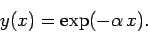
Consider the following example. Suppose that our o.d.e. is
 |
(14) |
where  , subject to the boundary condition
 |
(15) |
Of course, we can solve this problem analytically to give
 |
(16) |
Note that the solution is a monotonically decreasing function of  .
We can also solve this problem numerically using Euler's method. Appropriate
grid-points are
.
We can also solve this problem numerically using Euler's method. Appropriate
grid-points are
 |
(17) |
where
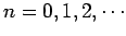 . Euler's method yields
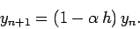 |
(18) |
Note one curious fact. If  then
then
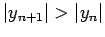 .
In other words, if the step-length is made too large then the numerical
solution becomes an oscillatory function of of
monotonically increasing amplitude:
i.e., the numerical solution diverges from the actual
solution. This type of catastrophic failure of a numerical integration
scheme is called a numerical instability. All simple integration
schemes become unstable if the step-length is made sufficiently large.
.
In other words, if the step-length is made too large then the numerical
solution becomes an oscillatory function of of
monotonically increasing amplitude:
i.e., the numerical solution diverges from the actual
solution. This type of catastrophic failure of a numerical integration
scheme is called a numerical instability. All simple integration
schemes become unstable if the step-length is made sufficiently large.
Next: Runge-Kutta methods
Up: Integration of ODEs
Previous: Numerical errors
Richard Fitzpatrick
2006-03-29