The CAM graphics class

There are a myriad of useful, prewritten C++ classes which are freely available on the web--for more details see http://www.trumphurst.com/cpplibsx.html. In this Subsection, we shall discuss just one of these--namely, the CAM graphics class,¹² whose purpose is to enable a C++ program to generate simple line plots. This class is freely available from the following URL: http://www.math.ucla.edu/~anderson/CAMclass/CAMClass.html

The CAM graphics class actually generates a PostScript¹³ file. Postscript is a programming language that describes the appearance of a printed page. It was developed by Adobe in 1985, and has become an industry standard for printing and imaging. All major printer manufacturers make printers that can interpret PostScript. A PostScript file is conventionally identified via a .ps suffix. The schematic code listed below illustrates the basic use of the CAM graphics class:

. . .
#include <gprocess.h> // Header file for CAM graphic class
. . .
CAMgraphicsProcess Gprocess;                 // declare a graphics process
CAMpostScriptDriver Pdriver("filename.ps");  // declare a PostScript driver
Gprocess.attachDriver(Pdriver);              // attach driver to process
. . .
Gprocess.frame();                            // "frame" the first plot
. . .
Gprocess.frame();                            // "frame" the second plot
. . .
. . .  
Gprocess.frame();                            // "frame" the last plot
Gprocess.detachDriver();                     // detach the driver
. . .

The header file for the class is called gprocess.h. The procedure for generating a plot is to first declare a graphics process, then declare a PostScript driver and attach this to a PostScript file--filename.ps, in the above example--and, finally, attach this driver to the process. A PostScript file can contain multiple pictures, or frames. Each frame is terminated by a call to Gprocess.frame(). Finally, the driver is detached, which has the effect of closing the PostScript file.

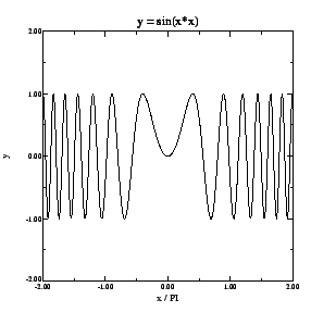
The program listed below uses the CAM graphics class to plot the curve $y=\sin^2 x$ for $x$ in the range $-2\pi$ to $2\pi$.

/* camgraph1.cpp */
/*
  Illustration of use of CAM graphics class to create simple line plot

  Program plots y = sin^2 x versus x in range -2 PI to +2 PI

  Program adapted from gpsmp1.cpp by Chris Anderson, UCLA 1996
*/

#include <gprocess.h>
#include <math.h>
#include <stdlib.h>

double func(double);

int main()
{
  int N_points = 400;
  double x_start = -2. * M_PI;                
  double x_end = 2. * M_PI; 
  double delta_x = (x_end - x_start) / ((double) N_points - 1.);

  double *x = new double[N_points];  
  double *y = new double[N_points];

  for (int i = 0; i < N_points; i++)
    {
      x[i] = x_start + (double) i * delta_x;
      y[i] = func(x[i]);
      x[i] /= M_PI;
    }

  { // This brace used to limit scope of Gprocess
    CAMgraphicsProcess Gprocess;                // declare a graphics process
    CAMpostScriptDriver Pdriver("graph1.ps");   // declare a PostScript driver
    Gprocess.attachDriver(Pdriver);             // attach driver to process

    Gprocess.setAxisRange(-2., 2., -2., 2.);    // set plotting ranges
    Gprocess.title("y = sin(x*x)");             // label the plot
    Gprocess.labelX("x / PI");
    Gprocess.labelY("y");

    Gprocess.plot(x, y, N_points);              // do the plotting

    Gprocess.frame();                           // "frame" the plot

    Gprocess.detachDriver();                    // detach the driver
  } // This brace calls the destructor for Gprocess:
    // without it the system() call would hang up

  delete[] x;	           
  delete[] y;

  system("gv graph1.ps");  // display plot on screen         

  return 0;
}

double func(double x)
{ 
  return sin(x*x);
}

The command Gprocess.plot(x, y, n) plots the n values of vector y against the n values of vector x as a solid curve. The command Gprocess.setAxisRange(x_low, x_high, y_low, y_high) sets the range of plotting. Finally, the commands Gprocess.title("title"), Gprocess.labelX("x_label"), and Gprocess.labelY("y_label") label the plot, the $x$-axis, and the $y$-axis, respectively. Incidentally, the UNIX function call system("gv graph1.ps") is used to pass the command gv graph1.ps to the operating system. On execution, this command displays the contents of graph1.ps on the screen. The graph written in the file graph1.ps is shown in Fig 1

Figure 1: An example plot generated by the CAM graphics class.

The program shown below illustrates some of the more advanced features of the CAM graphics class:

/* camgraph2.cpp */
/*
  Illustration of use of CAMgraphics class to create more advanced line plots

  Program plots three trigonometric functions versus x in range 
   -2 PI to +2 PI using different plot styles and different
   line styles

  Program adapted from gpsmp2.cpp by Chris Anderson, UCLA 1996
*/

#include <gprocess.h>
#include <math.h>
#include <stdlib.h>

double fun1(double);
double fun2(double);
double fun3(double);

int main()
{
  int N_points = 100;
  double x_start = -2. * M_PI;                
  double x_end = 2. * M_PI; 
  double delta_x = (x_end - x_start) / ((double) N_points - 1.);
  
  double *x  = new double[N_points];
  double *y1 = new double[N_points];
  double *y2 = new double[N_points];
  double *y3 = new double[N_points];

  for (int i = 0; i < N_points; i++)
    {
      x[i] = x_start + (double) i * delta_x;
      y1[i] = fun1(x[i]);
      y2[i] = fun2(x[i]);
      y3[i] = fun3(x[i]);
      x[i] /= M_PI;
    }

  {
    CAMgraphicsProcess Gprocess;              // declare a graphics process
    CAMpostScriptDriver Pdriver("graph2.ps"); // declare a PostScript driver
    Gprocess.attachDriver(Pdriver);           // attach driver to process
    
    /* First frame;  using different plot "styles" */
    Gprocess.setAxisRange(-2., 2., -2., 2.);            // set plotting ranges
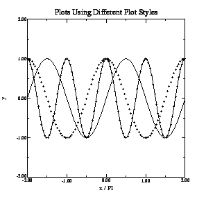
    Gprocess.title("Plots Using Different Plot Styles");// label the plot
    Gprocess.labelX("x / PI");
    Gprocess.labelY("y");

    Gprocess.plot(x, y1, N_points);              // solid line (default)
    Gprocess.plot(x, y2, N_points, '+');         // + markers
    Gprocess.plot(x, y3, N_points, '+', 2);      // + markers and solid line

    Gprocess.frame();                            // "frame" the plot

    /* Second frame; using different plot line "styles" */
    Gprocess.setAxisRange(-2., 2., -2., 2.);            // set plotting ranges
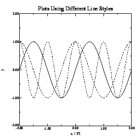
    Gprocess.title("Plots Using Different Line Styles");// label the plot
    Gprocess.labelX("x / PI");
    Gprocess.labelY("y");

    Gprocess.plot(x, y1, N_points);         // solid line (default)
    Gprocess.setPlotDashPattern(1);
    Gprocess.plot(x, y2, N_points);         // dashed line
    Gprocess.setPlotDashPattern(4);
    Gprocess.plot(x, y3, N_points);         // dashed-dot line

    Gprocess.frame();                       // "frame" the plot

    Gprocess.detachDriver();                // detach the driver
  }

  delete[] x;
  delete[] y1;
  delete[] y2;
  delete[] y3;

  system("gv graph2.ps"); // display plots on screen     
  
  return 0;
}

double fun1(double x)
{ 
  return sin(x);
}

double fun2(double x)
{ 
  return cos(x);
}

double fun3(double x)
{ 
  return cos(2.*x);
}

The command Gprocess.plot(x, y, n, '+') plots the n values of vector y against the n values of vector x as a set of points, each indicated by a '+' character. The command Gprocess.plot(x, y, n, '+', 2) does the same, but also connects the points with a solid line. The fourth argument of this command is an integer code which determines the plot style. The various options are as follows: 0 - curve; 1 - points; 2 - curve and points. The command Gprocess.setPlotDashPattern(n) sets the line style. The argument is again an integer code. The various options are: 0 - solid; 1 - dash; 2 - double-dash; 4 - dash-dot; 5 - dash-double-dot; 6 - dots.

The graphs written in the first and second frames of graph2.ps are shown in Figs. 2 and 3, respectively.

Figure 2: An example plot generated by the CAM graphics class.

Figure 3: An example plot generated by the CAM graphics class.