Consider ![]() atoms in the presence of a
atoms in the presence of a ![]() -directed magnetic field of
strength
-directed magnetic field of
strength ![]() . Suppose that all
atoms are identical spin-
. Suppose that all
atoms are identical spin-![]() systems. It follows that either
systems. It follows that either ![]() (spin up) or
(spin up) or ![]() (spin down), where
(spin down), where ![]() is (twice) the
is (twice) the ![]() -component
of the
-component
of the ![]() th atomic spin. The total energy of the system is
written:
th atomic spin. The total energy of the system is
written:
The physics of the Ising model is as follows. The first term on the right-hand
side of Eq. (351) shows that the overall energy is lowered when
neighbouring atomic spins are aligned. This effect is mostly
due to the Pauli exclusion principle. Electrons cannot occupy the same quantum
state, so two electrons on neighbouring atoms which have parallel spins
(i.e., occupy the same orbital state) cannot come close together in
space. No such restriction applies if the electrons have anti-parallel
spins. Different spatial separations imply different electrostatic
interaction energies, and the exchange energy, ![]() , measures this difference.
Note that since the exchange energy is electrostatic in origin, it
can be quite large: i.e.,
, measures this difference.
Note that since the exchange energy is electrostatic in origin, it
can be quite large: i.e., ![]() eV. This is far larger than the
energy associated with the direct magnetic interaction between neighbouring
atomic spins, which
is only about
eV. This is far larger than the
energy associated with the direct magnetic interaction between neighbouring
atomic spins, which
is only about ![]() eV. However, the exchange effect is very short-range; hence,
the restriction to nearest neighbour interaction is quite realistic.
eV. However, the exchange effect is very short-range; hence,
the restriction to nearest neighbour interaction is quite realistic.
Our first attempt to analyze the Ising model will employ a simplification
known as the mean field approximation. The energy of the ![]() th atom is written
th atom is written
 |
(352) |
 |
(353) |
We can write
| (354) |
 |
(355) |
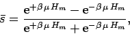
Consider a single atom in a magnetic field ![]() . Suppose that
the atom is in thermal equilibrium with a heat bath of temperature
. Suppose that
the atom is in thermal equilibrium with a heat bath of temperature
![]() . According to the well-known Boltzmann distribution, the mean spin
of the atom is
. According to the well-known Boltzmann distribution, the mean spin
of the atom is
 |
(356) |
Let us assume that all atoms have identical spins: i.e., ![]() .
This assumption is known as the ``mean field approximation''.
We can write
.
This assumption is known as the ``mean field approximation''.
We can write
| (360) |
 |
(361) |
| (362) |
It is helpful to define the net magnetization,
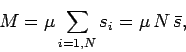 |
(364) |
 |
(365) |
| (366) |
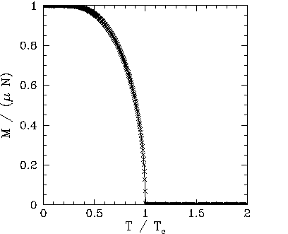 |
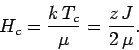
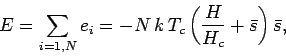
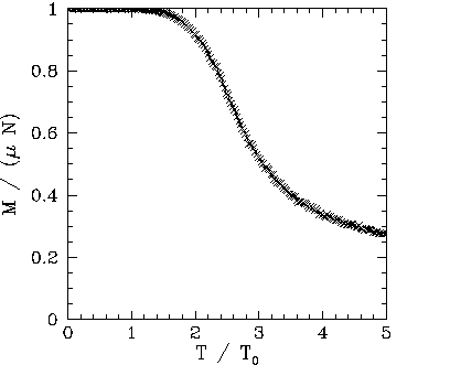
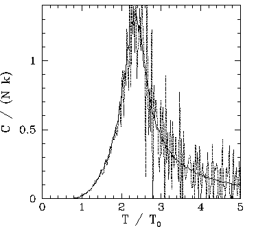
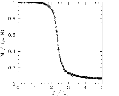
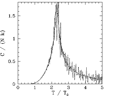
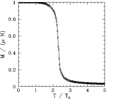
Figures 102, 101, and 103 show the net magnetization, net energy,
and heat capacity calculated from the iteration formula (363) in the
absence of an external magnetic field (i.e., with ![]() ). It
can be seen that below the critical (or ``Curie'') temperature,
). It
can be seen that below the critical (or ``Curie'') temperature, ![]() , there is
spontaneous magnetization: i.e., the exchange effect is sufficiently large
to cause neighbouring atomic spins to spontaneously align. On the other hand,
thermal fluctuations completely eliminate any alignment above the critical temperature. Moreover, at the
critical temperature there is a
discontinuity in the first derivative of the energy,
, there is
spontaneous magnetization: i.e., the exchange effect is sufficiently large
to cause neighbouring atomic spins to spontaneously align. On the other hand,
thermal fluctuations completely eliminate any alignment above the critical temperature. Moreover, at the
critical temperature there is a
discontinuity in the first derivative of the energy, ![]() , with respect to
the temperature,
, with respect to
the temperature, ![]() . This discontinuity generates a downward jump
in the heat capacity,
. This discontinuity generates a downward jump
in the heat capacity, ![]() , at
, at ![]() . The sudden loss of spontaneous
magnetization as the temperature exceeds the critical temperature is a type of
phase transition.
. The sudden loss of spontaneous
magnetization as the temperature exceeds the critical temperature is a type of
phase transition.
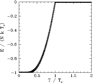 |
Now, according to the conventional classification of phase transitions, a transition is first-order if the energy is discontinuous with respect to the order parameter (i.e., in this case, the temperature), and second-order if the energy is continuous, but its first derivative with respect to the order parameter is discontinuous, etc. We conclude that the loss of spontaneous magnetization in a ferromagnetic material as the temperature exceeds the critical temperature is a second-order phase transition.
 |
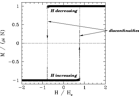
In order to see an example of a first-order phase transition, let us examine
the behaviour of the magnetization, ![]() , as the external field,
, as the external field, ![]() , is
varied at constant temperature,
, is
varied at constant temperature, ![]() .
.
 |
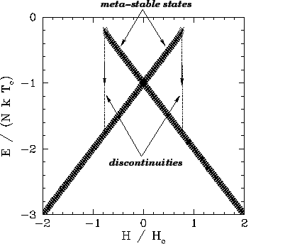 |
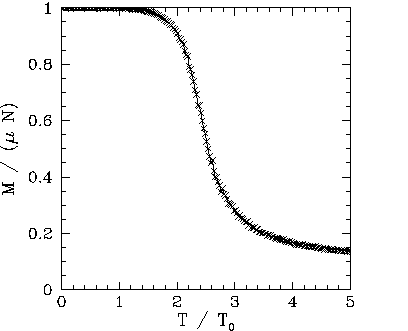
Figures 104 and 105 show the magnetization, ![]() , and energy,
, and energy, ![]() , versus
external field-strength,
, versus
external field-strength, ![]() , calculated from the iteration formula (363)
at some constant temperature,
, calculated from the iteration formula (363)
at some constant temperature, ![]() , which is less
than the critical temperature,
, which is less
than the critical temperature, ![]() . It can be seen that
. It can be seen that ![]() is
discontinuous, indicating the presence of a first-order phase transition.
Moreover, the system exhibits hysteresis--meta-stable
states exist within a certain range of
is
discontinuous, indicating the presence of a first-order phase transition.
Moreover, the system exhibits hysteresis--meta-stable
states exist within a certain range of ![]() values, and the magnetization of the system
at fixed
values, and the magnetization of the system
at fixed ![]() and
and ![]() (within the aforementioned range) depends on its past history:
i.e., on whether
(within the aforementioned range) depends on its past history:
i.e., on whether ![]() was increasing or decreasing when it entered the meta-stable
range.
was increasing or decreasing when it entered the meta-stable
range.
 |
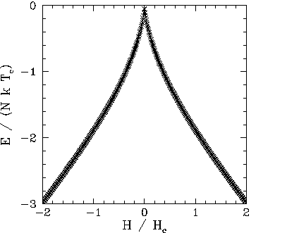 |
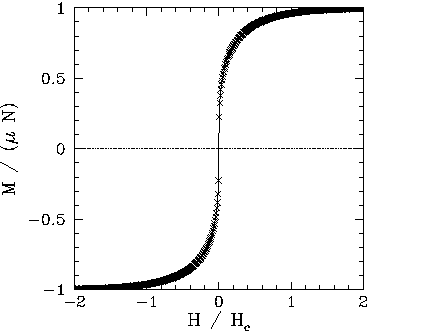
Figures 106 and 107 show the magnetization, ![]() , and energy,
, and energy, ![]() , versus
external field-strength,
, versus
external field-strength, ![]() , calculated from the iteration formula (363)
at a constant temperature,
, calculated from the iteration formula (363)
at a constant temperature, ![]() , which is equal to the critical temperature,
, which is equal to the critical temperature, ![]() .
It can be seen that
.
It can be seen that ![]() is now
continuous, and there are no meta-stable states. We conclude that first-order
phase transitions and hysteresis only occur, as the external field-strength is varied, when the
temperature lies below the critical temperature: i.e., when the ferromagnetic
material in question is capable of spontaneous magnetization.
is now
continuous, and there are no meta-stable states. We conclude that first-order
phase transitions and hysteresis only occur, as the external field-strength is varied, when the
temperature lies below the critical temperature: i.e., when the ferromagnetic
material in question is capable of spontaneous magnetization.
The above calculations, which are based on the mean field approximation, correctly predict
the existence of first- and second-order phase transitions when ![]() and
and ![]() ,
respectively. However, these calculations get some of the details of the second-order
phase transition wrong. In order to do a better job, we must abandon the mean
field approximation and
adopt a Monte-Carlo approach.
,
respectively. However, these calculations get some of the details of the second-order
phase transition wrong. In order to do a better job, we must abandon the mean
field approximation and
adopt a Monte-Carlo approach.
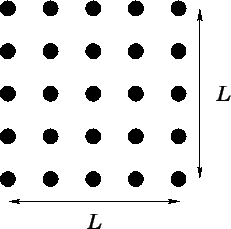
Let us consider a two-dimensional square array of atoms. Let ![]() be the
size of the array, and
be the
size of the array, and ![]() the number of atoms in the array, as shown in
Fig. 108. The Monte-Carlo approach to the Ising model, which completely avoids
the use of the mean field approximation, is based on the following
algorithm:
the number of atoms in the array, as shown in
Fig. 108. The Monte-Carlo approach to the Ising model, which completely avoids
the use of the mean field approximation, is based on the following
algorithm:
In order to demonstrate that the above algorithm is correct, let us consider
flipping the spin of the ![]() th atom. Suppose that this operation causes the
system to make a transition from state
th atom. Suppose that this operation causes the
system to make a transition from state ![]() (energy,
(energy, ![]() ) to state
) to state ![]() (energy,
(energy, ![]() ).
Suppose, further, that
).
Suppose, further, that ![]() . According to the above algorithm, the probability
of a transition from state
. According to the above algorithm, the probability
of a transition from state ![]() to state
to state ![]() is
is
| (367) |
| (368) |
| (370) |
Now, each atom in our array has four nearest neighbours, except for atoms on the edge of the array, which have less than four neighbours. We can eliminate this annoying special behaviour by adopting periodic boundary conditions: i.e., by identifying opposite edges of the array. Indeed, we can think of the array as existing on the surface of a torus.
It is helpful to define
| (371) |
| (372) |
 |
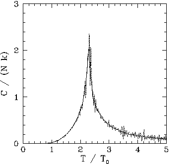
Figures 109-116 show magnetization and heat capacity versus temperature
curves for ![]() , 10, 20, and 40 in the absence of an
external magnetic field. In all cases, the Monte-Carlo simulation is iterated 5000 times,
and the first 1000 iterations are discarded when evaluating
, 10, 20, and 40 in the absence of an
external magnetic field. In all cases, the Monte-Carlo simulation is iterated 5000 times,
and the first 1000 iterations are discarded when evaluating ![]() (in order to
allow the system to attain thermal equilibrium). The two-dimensional array of atoms is
initialized in a fully aligned state for each different value of the temperature. Since there is
no external magnetic field, it is irrelevant whether the magnetization, M, is
positive or negative. Hence,
(in order to
allow the system to attain thermal equilibrium). The two-dimensional array of atoms is
initialized in a fully aligned state for each different value of the temperature. Since there is
no external magnetic field, it is irrelevant whether the magnetization, M, is
positive or negative. Hence, ![]() is replaced by
is replaced by ![]() in all plots.
in all plots.
 |
Note that the ![]() versus
versus ![]() curves generated by the Monte-Carlo simulations
look very much like those predicted by the
mean field model. The resemblance increases as the size,
curves generated by the Monte-Carlo simulations
look very much like those predicted by the
mean field model. The resemblance increases as the size, ![]() , of the atomic
array increases. The major difference is the presence of a magnetization ``tail'' for
, of the atomic
array increases. The major difference is the presence of a magnetization ``tail'' for ![]() in
the Monte-Carlo simulations: i.e., in the Monte-Carlo simulations the spontaneous magnetization
does not collapse to zero once the critical temperature is exceeded--there is
a small lingering magnetization for
in
the Monte-Carlo simulations: i.e., in the Monte-Carlo simulations the spontaneous magnetization
does not collapse to zero once the critical temperature is exceeded--there is
a small lingering magnetization for ![]() .
The
.
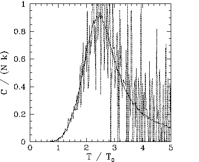
The ![]() versus
versus ![]() curves show the heat capacity calculated directly (i.e.,
curves show the heat capacity calculated directly (i.e.,
![]() ),
and via the identity
),
and via the identity
![]() . The latter method of calculation is
clearly far superior, since it generates significantly less statistical noise. Note that the heat capacity
peaks at the critical temperature: i.e., unlike the mean field model,
. The latter method of calculation is
clearly far superior, since it generates significantly less statistical noise. Note that the heat capacity
peaks at the critical temperature: i.e., unlike the mean field model, ![]() is
not zero for
is
not zero for ![]() . This effect is due to the residual magnetization present when
. This effect is due to the residual magnetization present when ![]() .
.
 |
Our best estimate for ![]() is obtained from the location of the peak in the
is obtained from the location of the peak in the ![]() versus
versus ![]() curve in Fig. 116. We obtain
curve in Fig. 116. We obtain ![]() . Recall that the mean field model
yields
. Recall that the mean field model
yields ![]() . The exact answer for a two-dimensional array of ferromagnetic atoms
is
. The exact answer for a two-dimensional array of ferromagnetic atoms
is
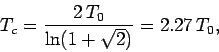 |
(375) |
 |
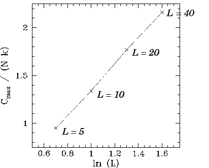
Note, from Figs. 110, 112, 114, and 116, that the height of the peak in the heat capacity curve at ![]() increases with increasing array
size,
increases with increasing array
size, ![]() . Indeed, a close examination of these figures yields
. Indeed, a close examination of these figures yields
![]() for
for ![]() ,
,
![]() for
for ![]() ,
,
![]() for
for ![]() , and
, and
![]() for
for ![]() .
Figure 117 shows
.
Figure 117 shows
![]() plotted against
plotted against ![]() for
for ![]() , 10, 20, and 40.
It can be seen that the points lie on a very convincing straight-line, which strongly suggests that
, 10, 20, and 40.
It can be seen that the points lie on a very convincing straight-line, which strongly suggests that
| (376) |
 |
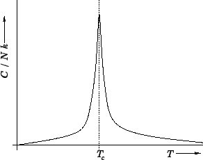
Of course, for physical systems,
![]() , where
, where ![]() is Avogadro's
number. Hence,
is Avogadro's
number. Hence, ![]() is effectively singular at the critical temperature
(since
is effectively singular at the critical temperature
(since ![]() ), as sketched in
Fig. 118. This observation leads us to revise our definition of a second-order phase
transition. It turns out that actual discontinuities in the heat capacity almost
never occur. Instead, second-order phase transitions are
characterized by a local quasi-singularity in the heat capacity.
), as sketched in
Fig. 118. This observation leads us to revise our definition of a second-order phase
transition. It turns out that actual discontinuities in the heat capacity almost
never occur. Instead, second-order phase transitions are
characterized by a local quasi-singularity in the heat capacity.
 |
Recall, from Eq. (374), that the typical amplitude of energy fluctuations is proportional
to the square-root of the heat capacity (i.e.,
![]() ). It
follows that the amplitude of energy fluctuations becomes extremely large in the vicinity
of a second-order phase transition.
). It
follows that the amplitude of energy fluctuations becomes extremely large in the vicinity
of a second-order phase transition.
 |
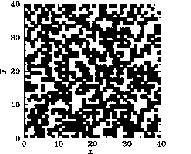
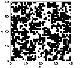
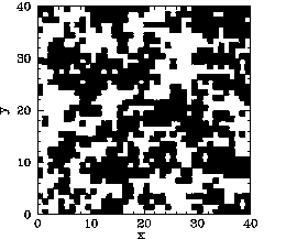
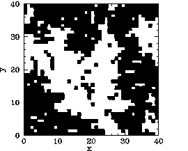
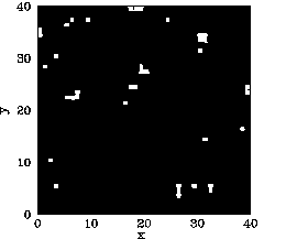
Now, the main difference between our mean field and Monte-Carlo calculations is the existence
of residual magnetization for ![]() in the latter case. Figures 119-123
show the magnetization pattern of a
in the latter case. Figures 119-123
show the magnetization pattern of a ![]() array of ferromagnetic atoms, in thermal
equilibrium and in the absence of an external magnetic field, calculated at various temperatures.
It can be seen that for
array of ferromagnetic atoms, in thermal
equilibrium and in the absence of an external magnetic field, calculated at various temperatures.
It can be seen that for ![]() the pattern is essentially random. However,
for
the pattern is essentially random. However,
for ![]() , small clumps appear in the pattern. For
, small clumps appear in the pattern. For ![]() , the clumps
are somewhat bigger. For
, the clumps
are somewhat bigger. For ![]() , which is just above the critical temperature,
the clumps are global in extent. Finally, for
, which is just above the critical temperature,
the clumps are global in extent. Finally, for ![]() , which is a little
below the critical temperature, there is almost complete alignment of the atomic spins.
, which is a little
below the critical temperature, there is almost complete alignment of the atomic spins.
 |
The problem with the mean field model is that it assumes that all atoms are situated in identical environments. Hence, if the exchange effect is not sufficiently large to cause global alignment of the atomic spins then there is no alignment at all. What actually happens when the temperature exceeds the critical temperature is that global alignment disappears, but local alignment (i.e., clumping) remains. Clumps are only eliminated by thermal fluctuations once the temperature is significantly greater than the critical temperature. Atoms in the middle of the clumps are situated in a different environment than atoms on the clump boundaries. Hence, clumps cannot occur in the mean field model.
 |
 |
 |
 |
 |
 |
 |