Distribution functions

Let $P(x)\,dx$ represent the probability of finding the random variable $x$ in the interval $x$ to $x+dx$. Here, $P(x)$ is termed a probability density. Note that $P=0$ corresponds to no chance, whereas $P=1$ corresponds to certainty. Since it is certain that the value of $x$ lies in the range $-\infty$ to $+\infty$, probability densities are subject to the normalizing constraint

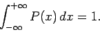$$\int_{-\infty}^{+\infty} P(x)\,dx = 1.$$ (315)

Suppose that we wish to construct a random variable $x$ which is uniformly distributed in the range $x_1$ to $x_2$. In other words, the probability density of $x$ is

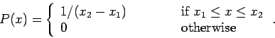$$P(x) = \left\{\begin{array}{lcl} 1/(x_2-x_1) &\mbox{\hspace{... ... \leq x \leq x_2$}\\ 0&& \mbox{otherwise} \end{array}\right..$$ (316)

Such a variable is constructed as follows

x = x1 + (x2 - x1) * double (random ()) / double (RANDMAX);

There are two basic methods of constructing non-uniformly distributed random variables: i.e., the transformation method and the rejection method. We shall examine each of these methods in turn.

Let us first consider the transformation method. Let $y=f(x)$, where $f$ is a known function, and $x$ is a random variable. Suppose that the probability density of $x$ is $P_x(x)$. What is the probability density, $P_y(y)$, of $y$? Our basic rule is the conservation of probability:

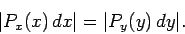$$\vert P_x(x)\,dx\vert = \vert P_y(y)\,dy\vert.$$ (317)

In other words, the probability of finding $x$ in the interval $x$ to $x+dx$ is the same as the probability of finding $y$ in the interval $y$ to $y+dy$. It follows that

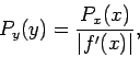$$P_y(y) = \frac{P_x(x)}{\vert f'(x)\vert},$$ (318)

where $f'=df/dx$.

For example, consider the Poisson distribution:

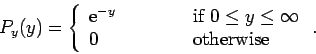$$P_y(y) = \left\{\begin{array}{lcl} {\rm e}^{-y}&\mbox{\hspac... ...eq y \leq \infty$}\\ 0&& \mbox{otherwise} \end{array}\right..$$ (319)

Let $y=f(x)=-\ln x$, so that $\vert f'\vert = 1/x$. Suppose that

$$P_x(x) = \left\{\begin{array}{lcl} 1&\mbox{\hspace{1cm}}&\mb... ...$0 \leq x \leq 1$}\\ 0&& \mbox{otherwise} \end{array}\right..$$ (320)

It follows that

$$P_y(y) = \frac{1}{\vert f'\vert}= x = {\rm e}^{-y},$$ (321)

with $x=0$ corresponding to $y=\infty$, and $x=1$ corresponding to $y=0$. We conclude that if

x = double (random ()) / double (RANDMAX);
y = - log (x);

then y is distributed according to the Poisson distribution.

The transformation method requires a differentiable probability distribution function. This is not always practical. In such cases, we can use the rejection method instead.

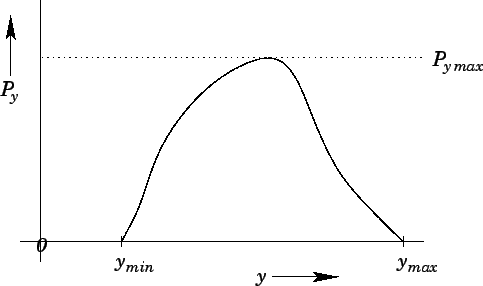
Suppose that we desire a random variable $y$ distributed with density $P_y(y)$ in the range $y_{\rm min}$ to $y_{\rm max}$. Let $P_{y\,{\rm max}}$ be the maximum value of $P(y)$ in this range (see Fig. 95). The rejection method is as follows. The variable $y$ is sampled randomly in the range $y_{\rm min}$ to $y_{\rm max}$. For each value of $y$ we first evaluate $P_y(y)$. We next generate a random number $x$ which is uniformly distributed in the range 0 to $P_{y\,{\rm max}}$. Finally, if $P_y(y) < x$ then we reject the $y$ value; otherwise, we keep it. If this prescription is followed then $y$ will be distributed according to $P_y(y)$.

Figure 95: The rejection method.

As an example, consider the Gaussian distribution:

$$P_y(y) =\frac{{\rm exp}[(y-\bar{y})^2/2\,\sigma^2]}{\sqrt{2\pi}\,\sigma},$$ (322)

where $\bar{y}$ is the mean value of $y$, and $\sigma$ is the standard deviation. Let

$$y_{\rm min} = \bar{y}-4\,\sigma,$$ (323)

$$y_{\rm max} = \bar{y}+4\,\sigma,$$ (324)

since there is a negligible chance that $y$ lies more than 4 standard deviations from its mean value. It follows that

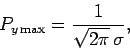$$P_{y\,{\rm max}} = \frac{1}{\sqrt{2\pi}\,\sigma},$$ (325)

with the maximum occurring at $y=\bar{y}$. The function listed below employs the rejection method to return a random variable distributed according to a Gaussian distribution with mean mean and standard deviation sigma:

// gaussian.cpp

// Function to return random variable distributed
// according to Gaussian distribution with mean mean
// and standard deviation sigma.

#define RANDMAX 2147483646

int random (int = 0);

double gaussian (double mean, double sigma)
{
  double ymin = mean - 4. * sigma;
  double ymax = mean + 4. * sigma;
  double Pymax = 1. / sqrt (2. * M_PI) / sigma;

  // Calculate random value uniformly distributed 
  //  in range ymin to ymax
  double y = ymin + (ymax - ymin) * double (random ()) / double (RANDMAX);

  // Calculate Py
  double Py = exp (- (y - mean) * (y - mean) / 2. / sigma / sigma) /
    sqrt (2. * M_PI) / sigma;

  // Calculate random value uniformly distributed in range 0 to Pymax
  double x = Pymax * double (random ()) / double (RANDMAX);

  // If x > Py reject value and recalculate
  if (x > Py) return gaussian (mean, sigma);
  else return y;
}

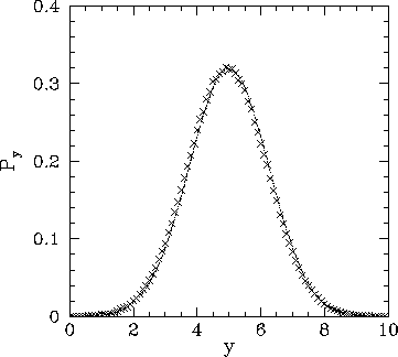
Figure 96 illustrates the performance of the above function. It can be seen that the function successfully returns a random value distributed according to the Gaussian distribution.

Figure: A million values returned by function gaussian with mean = 5. and sigma = 1.25. The values are binned in 100 bins of width 0.1. The figure shows the number of points in each bin divided by a suitable normalization factor. A Gaussian curve is shown for comparison.