


Next: Vector Area
Up: Vectors
Previous: Vectors
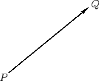
Figure 1:
A directed line element.
 |
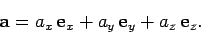
In applied mathematics, physical quantities are (predominately) represented by two distinct classes
of objects. Some quantities, denoted scalars, are represented by real
numbers. Others, denoted vectors, are represented by
directed line elements in space: e.g.,
 in see Fig. 1.
Note that line elements
(and, therefore, vectors) are movable, and do not carry intrinsic position information: i.e., in Fig. 2,
in see Fig. 1.
Note that line elements
(and, therefore, vectors) are movable, and do not carry intrinsic position information: i.e., in Fig. 2,
 and
and
 are considered to be the same vector.
In fact, vectors just possess a magnitude and a direction, whereas scalars possess
a magnitude but no direction.
By convention, vector quantities are denoted by bold-faced characters (e.g.,
are considered to be the same vector.
In fact, vectors just possess a magnitude and a direction, whereas scalars possess
a magnitude but no direction.
By convention, vector quantities are denoted by bold-faced characters (e.g.,
 ) in
typeset documents.
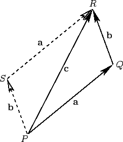
Vector addition
can be represented using a parallelogram: e.g.,
) in
typeset documents.
Vector addition
can be represented using a parallelogram: e.g.,
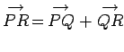 in Fig. 2.
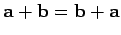
 is said to be the resultant of
and
.
Suppose that
is said to be the resultant of
and
.
Suppose that
 ,
,
 , and
, and
 . It follows,
from Fig. 2, that vector addition is
commutative: i.e.,
. It follows,
from Fig. 2, that vector addition is
commutative: i.e.,
 (since
is also the resultant
of
and
(since
is also the resultant
of
and
 ). It can also
be shown that the associative law holds: i.e.,
). It can also
be shown that the associative law holds: i.e.,
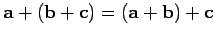 .
.
Figure 2:
Vector addition.
 |
There are two general approaches to vector analysis. The geometric approach is
based on drawing line elements in space, and then making use
of the theorems of Euclidian geometry. The coordinate approach assumes that
space is defined by Cartesian coordinates, and uses these to characterize vectors.
In Physics, we generally
adopt the second approach, because it is far more convenient.
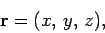
In the coordinate approach, a vector is denoted as the row matrix of
its components along each of the Cartesian axes (the  -,
-,  -, and
  -axes, say):
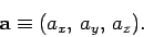 |
(1) |
Here,  is the -coordinate of the ``head'' of the vector minus
the -coordinate of its ``tail,'' etc.
If
is the -coordinate of the ``head'' of the vector minus
the -coordinate of its ``tail,'' etc.
If
 and
and
 then vector addition is defined
 |
(2) |
If is a vector and  is a scalar then the product
of a scalar and a vector is defined
is a scalar then the product
of a scalar and a vector is defined
 |
(3) |
The vector  is interpreted as a vector which points
in the same direction as (or in the opposite
direction, if
is interpreted as a vector which points
in the same direction as (or in the opposite
direction, if  ), and is
  times as long as .
It is clear that vector algebra is distributive with respect to
scalar multiplication: i.e.,
times as long as .
It is clear that vector algebra is distributive with respect to
scalar multiplication: i.e.,
 .
.
Unit vectors can be defined in the -, -, and -directions as
 ,
,
 , and
, and
 . Any vector can be written in terms of these unit vectors: i.e.,
 |
(4) |
In mathematical terminology,
three vectors used in this manner form a basis of the vector space. If the
three vectors are mutually perpendicular then they are termed orthogonal basis
vectors. However, any set of three non-coplanar vectors can be used as basis
vectors.
Examples of vectors in Physics are displacements from an origin,
 |
(5) |
and velocities,
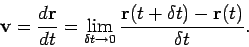 |
(6) |
Figure 3:
Rotation of the basis about the -axis.
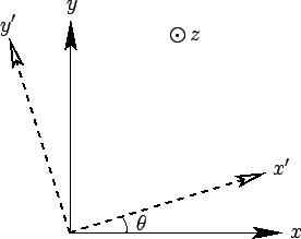 |
Suppose that we transform to a new orthogonal basis, the  -,
-,  -, and
  -axes,
which are related to the -, -, and -axes via a rotation through an angle
-axes,
which are related to the -, -, and -axes via a rotation through an angle
 around the -axis--see Fig. 3.
In the new basis, the coordinates of the general displacement
around the -axis--see Fig. 3.
In the new basis, the coordinates of the general displacement  from the
origin are
from the
origin are  . These coordinates are related to the previous
coordinates via the transformation
. These coordinates are related to the previous
coordinates via the transformation
Now, we do not need to change our notation for the displacement in the new basis.
It is still denoted . The reason for this is that the magnitude and
direction of are independent of the choice of basis vectors. The
coordinates of do depend on the choice of basis vectors.
However, they must depend in a very specific manner [i.e., Eqs. (7)-(9)] which
preserves the magnitude and direction of .
Since any vector can be represented as a displacement from an origin
(this is just a special case of a directed line element), it follows that
the
components of a general vector must transform in an similar
manner to Eqs. (7)-(9). Thus,
with analogous transformation rules for rotation about the - and -axes.
In the coordinate approach, Eqs. (10)-(12) constitute the definition of a vector.
The three
quantities (,  ,
,  ) are the components of a vector provided that
they transform under rotation like Eqs. (10)-(12).
Conversely, (, , ) cannot be the components of a vector if they
do not transform like Eqs. (10)-(12). Scalar quantities are invariant
under transformation.
Thus, the individual components of a vector (, say) are real numbers, but
they are
not scalars.
Displacement vectors, and all vectors derived from
displacements, automatically satisfy Eqs. (10)-(12). There are, however, other
physical quantities which have both magnitude and direction, but which are not
obviously related to displacements. We need to check carefully to see whether these
quantities are vectors.
) are the components of a vector provided that
they transform under rotation like Eqs. (10)-(12).
Conversely, (, , ) cannot be the components of a vector if they
do not transform like Eqs. (10)-(12). Scalar quantities are invariant
under transformation.
Thus, the individual components of a vector (, say) are real numbers, but
they are
not scalars.
Displacement vectors, and all vectors derived from
displacements, automatically satisfy Eqs. (10)-(12). There are, however, other
physical quantities which have both magnitude and direction, but which are not
obviously related to displacements. We need to check carefully to see whether these
quantities are vectors.
Next: Vector Area
Up: Vectors
Previous: Vectors
Richard Fitzpatrick
2007-07-14