Next: Multi-Slit Interference Up: Wave Optics Previous: Two-Slit Interference Contents
 , where
 is the difference in energy between the excited state
and the ground state, and
is the difference in energy between the excited state
and the ground state, and
 is Planck's constant divided by
  (Hecht and Zajac 1974).
An excited electronic state of an atom has a characteristic lifetime,
(Hecht and Zajac 1974).
An excited electronic state of an atom has a characteristic lifetime,  , which can be
calculated from quantum mechanics, and is typically
, which can be
calculated from quantum mechanics, and is typically
 (ibid.). It follows that when an atom in
an excited state decays back to its ground state it emits a burst of electromagnetic radiation of duration and angular frequency
(ibid.). It follows that when an atom in
an excited state decays back to its ground state it emits a burst of electromagnetic radiation of duration and angular frequency  .
However, according to the bandwidth theorem (see Section 8.5), a sinusoidal wave of finite duration has the finite bandwidth
.
However, according to the bandwidth theorem (see Section 8.5), a sinusoidal wave of finite duration has the finite bandwidth
 |
(10.21) |
 to
to
 .
We conclude that there is no such thing as a truly monochromatic light source. In reality, all such sources have small, but finite, bandwidths
that are inversely proportional to the lifetimes, , of the associated excited atomic states.
.
We conclude that there is no such thing as a truly monochromatic light source. In reality, all such sources have small, but finite, bandwidths
that are inversely proportional to the lifetimes, , of the associated excited atomic states.
How do we take the finite bandwidth of a practical “monochromatic” light source into account in our analysis? In fact,
all we need to do is to assume that the phase angle,  , appearing in Equations (10.1) and (10.15), is
only constant on timescales much less that the lifetime, , of the associated excited atomic state, and is subject to abrupt random changes on timescales much
greater than . We can understand this phenomenon as being due to the fact that the radiation emitted by a single atom has a
fixed phase angle, , but only lasts a finite time period, , combined with the fact that there is generally no correlation between the
phase angles of the radiation emitted by different atoms. Alternatively, we can account for the variation in the phase
angle in terms of the finite bandwidth of the light source. To be more exact, because the light emitted by the source consists of a superposition of sinusoidal waves of
frequencies extending over the range
to
, even if all the
component waves start off in phase, the phases will be completely scrambled after a time period
, appearing in Equations (10.1) and (10.15), is
only constant on timescales much less that the lifetime, , of the associated excited atomic state, and is subject to abrupt random changes on timescales much
greater than . We can understand this phenomenon as being due to the fact that the radiation emitted by a single atom has a
fixed phase angle, , but only lasts a finite time period, , combined with the fact that there is generally no correlation between the
phase angles of the radiation emitted by different atoms. Alternatively, we can account for the variation in the phase
angle in terms of the finite bandwidth of the light source. To be more exact, because the light emitted by the source consists of a superposition of sinusoidal waves of
frequencies extending over the range
to
, even if all the
component waves start off in phase, the phases will be completely scrambled after a time period
 has
elapsed. In effect, what we are saying is that a practical monochromatic light source is temporally coherent on timescales
much less than its characteristic coherence time, (which, for visible light, is typically
of order
has
elapsed. In effect, what we are saying is that a practical monochromatic light source is temporally coherent on timescales
much less than its characteristic coherence time, (which, for visible light, is typically
of order  seconds), and temporally incoherent on timescales much greater than . Incidentally, two waves are said
to be coherent if their phase difference is constant in time, and incoherent if their phase difference varies
significantly in time. In this case, the
two waves in question are the same wave observed at two different times.
seconds), and temporally incoherent on timescales much greater than . Incidentally, two waves are said
to be coherent if their phase difference is constant in time, and incoherent if their phase difference varies
significantly in time. In this case, the
two waves in question are the same wave observed at two different times.
What effect does the temporal incoherence of a practical monochromatic light source on timescales greater than
 seconds have on the two-slit interference patterns discussed in the previous section? Consider the case of oblique incidence.
According to Equation (10.16),
the phase angles,
seconds have on the two-slit interference patterns discussed in the previous section? Consider the case of oblique incidence.
According to Equation (10.16),
the phase angles,
 , and
, and
 , of the
cylindrical waves emitted by each slit are subject to abrupt random changes on timescales much greater than , because the
phase angle, , of the plane wave that illuminates the two slits is subject to identical changes. Nevertheless, the
relative phase angle,
, of the
cylindrical waves emitted by each slit are subject to abrupt random changes on timescales much greater than , because the
phase angle, , of the plane wave that illuminates the two slits is subject to identical changes. Nevertheless, the
relative phase angle,
 , between the two cylindrical waves remains constant. Moreover,
according to Equation (10.17), the interference pattern appearing on the projection screen is produced by the
phase difference
, between the two cylindrical waves remains constant. Moreover,
according to Equation (10.17), the interference pattern appearing on the projection screen is produced by the
phase difference
 between the two cylindrical waves at a given point on the screen,
and this phase difference only depends on the relative phase angle. Indeed, the
intensity of the interference pattern is
between the two cylindrical waves at a given point on the screen,
and this phase difference only depends on the relative phase angle. Indeed, the
intensity of the interference pattern is
![${\cal I}(\theta)\propto \cos^2[(1/2)\,k\,d\,\sin\theta-(1/2)\,(\phi_1-\phi_2)]$](img3323.png) .
Hence, the
fact that the relative phase angle,
.
Hence, the
fact that the relative phase angle,
 , between the two cylindrical waves emitted by the slits remains constant on timescales much
longer than the characteristic coherence time, , of the light source implies that the interference pattern generated in
a conventional two-slit interference apparatus
is unaffected by the temporal incoherence of the source. Strictly speaking, however, the preceding
conclusion is only accurate when the spatial extent of the light source is negligible. Let us now broaden
our discussion to take spatially extended light sources into account.
, between the two cylindrical waves emitted by the slits remains constant on timescales much
longer than the characteristic coherence time, , of the light source implies that the interference pattern generated in
a conventional two-slit interference apparatus
is unaffected by the temporal incoherence of the source. Strictly speaking, however, the preceding
conclusion is only accurate when the spatial extent of the light source is negligible. Let us now broaden
our discussion to take spatially extended light sources into account.
Up until now, we have assumed that our two-slit interference apparatus is illuminated by a single plane wave, such as
might be generated by a line source located at infinity. Let us now consider a more realistic situation in
which the light source is located a finite distance from the slits, and also has a finite spatial
extent. Figure 10.6 shows the simplest possible case. Here, the slits are
illuminated by two identical line sources,  and
and  , that are a distance
  apart, and a
perpendicular distance
apart, and a
perpendicular distance  from the opaque screen containing the slits. Assuming that
 , the
light incident on the slits from source is effectively a plane wave whose direction of propagation subtends an angle
, the
light incident on the slits from source is effectively a plane wave whose direction of propagation subtends an angle
 with the
  -axis. Likewise, the light incident on the slits from source is
a plane wave whose direction of propagation subtends an angle
-axis. Likewise, the light incident on the slits from source is
a plane wave whose direction of propagation subtends an angle
 with the -axis. Moreover, the net interference
pattern (i.e., wavefunction) appearing on the projection screen is the linear superposition of the patterns generated by each
source taken individually (because light propagation is ultimately governed by a linear
wave equation with superposable solutions; see Section 7.3.). Let us determine whether these patterns reinforce, or interfere with,
one another.
with the -axis. Moreover, the net interference
pattern (i.e., wavefunction) appearing on the projection screen is the linear superposition of the patterns generated by each
source taken individually (because light propagation is ultimately governed by a linear
wave equation with superposable solutions; see Section 7.3.). Let us determine whether these patterns reinforce, or interfere with,
one another.
The light emitted by source has a phase angle,  , that is constant on timescales
much less than the characteristic coherence time of the source, , but is subject to
abrupt random changes on timescale much longer than . Likewise, the light
emitted by source has a phase angle,
, that is constant on timescales
much less than the characteristic coherence time of the source, , but is subject to
abrupt random changes on timescale much longer than . Likewise, the light
emitted by source has a phase angle,  , that is constant on timescales much
less than , and varies significantly on timescales much greater than . In general, there is
no correlation between and . In other words, our composite
light source, consisting of the two line sources and , is both temporally and spatially
incoherent on timescales much longer than .
, that is constant on timescales much
less than , and varies significantly on timescales much greater than . In general, there is
no correlation between and . In other words, our composite
light source, consisting of the two line sources and , is both temporally and spatially
incoherent on timescales much longer than .
Again working in the limit
 , with
 , Equation (10.18) yields the following expression
for the wavefunction at the projection screen:
, Equation (10.18) yields the following expression
for the wavefunction at the projection screen:
 |
![$\displaystyle \propto \cos(\omega\,t-k\,R-\phi_A)\,\cos\left[\frac{1}{2}\,k\,d\,(\theta-\theta_0/2)\right]$](img3332.png) |
|
![$\displaystyle ~~~~+ \cos(\omega\,t-k\,R-\phi_B)\,\cos\left[\frac{1}{2}\,k\,d\,(\theta+\theta_0/2)\right].$](img3333.png) |
(10.22) |
 |
![$\displaystyle \propto \langle\,\cos^2 (\omega\,t-k\,R-\phi_A)\rangle\cos^2\left[\frac{1}{2}\,k\,d\,(\theta-\theta_0/2)\right]$](img3335.png) |
|
 |
||
![$\displaystyle \times \cos\left[\frac{1}{2}\,k\,d\,(\theta-\theta_0/2)\right]\,\cos\left[\frac{1}{2}\,k\,d\,(\theta+\theta_0/2)\right]$](img3337.png) |
||
![$\displaystyle ~~~~+\langle\,\cos^2 (\omega\,t-k\,R-\phi_B)\rangle\cos^2\left[\frac{1}{2}\,k\,d\,(\theta+\theta_0/2)\right].$](img3338.png) |
(10.23) |
 , and
, and
 , because the phase angles and
are uncorrelated. Hence, the previous expression reduces to
where use has been made of the trigonometric identities
, because the phase angles and
are uncorrelated. Hence, the previous expression reduces to
where use has been made of the trigonometric identities
 , and
, and
![$\cos x + \cos y \equiv 2\,\cos[(x+y)/2]\,\cos((x-y)/2]$](img3345.png) . (See Appendix B.)
If
. (See Appendix B.)
If
 then
then
![$\cos[\pi\,(d/\lambda)\,\theta_0]=0$](img3347.png) and
and
 .
In this case, the bright fringes of the interference pattern generated by source exactly overlay the dark fringes
of the pattern generated by source , and vice versa, and the net interference pattern is completely
washed out. On the other hand, if
.
In this case, the bright fringes of the interference pattern generated by source exactly overlay the dark fringes
of the pattern generated by source , and vice versa, and the net interference pattern is completely
washed out. On the other hand, if
 then
then
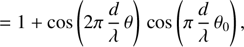
![$\cos[\pi\,(d/\lambda)\,\theta_0]\simeq 1$](img3350.png) and
and
![${\cal I}(\theta)\propto 1+\cos[2\pi\,(d/\lambda)\,\theta]=2\, \cos^2[\pi\,(d/\lambda)\,\theta]$](img3351.png) . In this case, the two interference patterns
reinforce one another, and the net interference pattern is the same as that generated by a light source
of negligible spatial extent.
. In this case, the two interference patterns
reinforce one another, and the net interference pattern is the same as that generated by a light source
of negligible spatial extent.
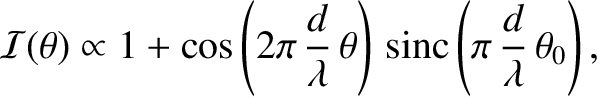
Suppose that our light source consists of a regularly spaced array of very many identical incoherent line sources, filling the region
between the sources and in Figure 10.6. In other words, suppose that our light source is a uniform incoherent source of
angular extent  .
As is readily demonstrated, the associated interference pattern is obtained
by averaging expression (10.24) over all values in the range 0 to ;
that is, by operating on this expression with
.
As is readily demonstrated, the associated interference pattern is obtained
by averaging expression (10.24) over all values in the range 0 to ;
that is, by operating on this expression with
 . In this manner,
we obtain
. In this manner,
we obtain
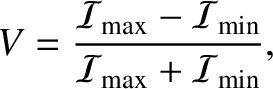
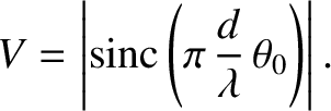
 . We can conveniently parameterize the visibility of the interference pattern, appearing on the projection
screen, in terms of the quantity
where the maximum and minimum values of the intensity are taken with respect to variation in
. We can conveniently parameterize the visibility of the interference pattern, appearing on the projection
screen, in terms of the quantity
where the maximum and minimum values of the intensity are taken with respect to variation in  (rather than ). Thus,
  corresponds to a sharply defined pattern, and
  to a pattern that is completely
washed out. It follows from Equation (10.25) that
to a pattern that is completely
washed out. It follows from Equation (10.25) that
 |
(10.27) |
 , of a two-slit interference pattern generated by an extended incoherent light source is plotted as a function of the angular extent, , of the source
in Figure 10.7. It can be seen that the pattern is highly visible (i.e.,
, of a two-slit interference pattern generated by an extended incoherent light source is plotted as a function of the angular extent, , of the source
in Figure 10.7. It can be seen that the pattern is highly visible (i.e.,  ) when
, but
becomes washed out (i.e.,
) when
, but
becomes washed out (i.e.,  ) when
 .
.
![\includegraphics[width=0.9\textwidth]{Chapter10/fig10_07.eps}](img3361.png) |
We conclude that a spatially extended incoherent light source only generates a visible interference pattern in a conventional two-slit interference apparatus when the angular extent of the source is sufficiently small that
 |
(10.28) |
, and located a distance from the slits, then the source
only generates a visible interference pattern when it is sufficiently far away from the slits that
 |
(10.29) |
 .
.
The whole of the preceding discussion is premised on the assumption that an extended light source is both
temporally and spatially incoherent on timescales much longer than a typical atomic coherence time, which is about seconds. This
is generally the case. However, there is one type of light source—namely, a laser—for which this is not necessarily the
case. In a laser (in single-mode operation), excited atoms are stimulated
in such a manner that they emit radiation that is both temporally and spatially coherent on timescales
much longer than the relevant atomic coherence time.
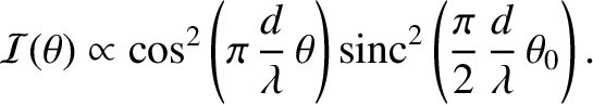
Let us consider the two-slit far-field interference pattern generated by an extended coherent light source of angular extent .
In this case, as is readily demonstrated (see Exercise 2), Equation (10.25) is replaced by
.)
It follows that lasers generally produce much clearer interference patterns than conventional incoherent light sources.
![\includegraphics[width=1\textwidth]{Chapter10/fig10_06.eps}](img3325.png)

![$\displaystyle \propto\cos^2\left[\frac{1}{2}\,k\,d\,(\theta-\theta_0/2)\right]+ \cos^2\left[\frac{1}{2}\,k\,d\,(\theta+\theta_0/2)\right]$](img3342.png)