Next: Exercises Up: Damped and Driven Harmonic Previous: Driven LCR Circuit Contents
 |
![$\displaystyle = \frac{\omega_0^{\,2}\,\hat{X}}{\left[(\omega_0^{\,2}-\omega^{\,2})^{\,2}+\nu^{\,2}\,\omega^{\,2}\right]^{1/2}},$](img590.png) |
(2.75) |
 |
 |
(2.76) |
 |
(2.77) |
 , and
, and  and
and  are arbitrary constants. [In terms of the standard solution, (2.12),
 and
and
 .]
Thus, a more general solution to Equation (2.73) is
In fact, because the preceding solution contains two arbitrary constants, we can be sure
that it is the most general solution. The arbitrary constants, and ,
are determined by the initial conditions. Thus, the
most general solution to the driven damped harmonic oscillator equation, (2.73),
consists of two parts: first, the solution (2.74), which oscillates at the driving frequency
.]
Thus, a more general solution to Equation (2.73) is
In fact, because the preceding solution contains two arbitrary constants, we can be sure
that it is the most general solution. The arbitrary constants, and ,
are determined by the initial conditions. Thus, the
most general solution to the driven damped harmonic oscillator equation, (2.73),
consists of two parts: first, the solution (2.74), which oscillates at the driving frequency  with a constant amplitude, and which is independent of the initial conditions; second, the
solution (2.78), which oscillates at the natural frequency
with a constant amplitude, and which is independent of the initial conditions; second, the
solution (2.78), which oscillates at the natural frequency  with an amplitude that decays exponentially in time, and
which depends on the initial conditions. The former is termed the
time asymptotic solution, because if we wait long enough then it
becomes dominant. The latter is called the transient solution, because if
we wait long enough then it decays away.
with an amplitude that decays exponentially in time, and
which depends on the initial conditions. The former is termed the
time asymptotic solution, because if we wait long enough then it
becomes dominant. The latter is called the transient solution, because if
we wait long enough then it decays away.
![\includegraphics[width=0.8\textwidth]{Chapter02/fig2_07.eps}](img594.png) |
Suppose, for the sake of argument, that the system is initially in its equilibrium
state. In other words,
 . It follows from Equation (2.79) that
 |
 |
(2.80) |
 |
 |
(2.81) |
 ), we
can write
), we
can write
|
![$\displaystyle \simeq \frac{\omega_0\,\hat{X}}{[4\,(\omega_0-\omega)^{\,2}+\nu^{\,2}]^{1/2}},$](img607.png) |
(2.84) |
 |
![$\displaystyle \simeq \frac{\nu}{[4\,(\omega_0-\omega)^{\,2}+\nu^{\,2}]^{1/2}},$](img608.png) |
(2.85) |
 |
![$\displaystyle \simeq \frac{2\,(\omega_0-\omega)}{[4\,(\omega_0-\omega)^{\,2}+\nu^{\,2}]^{1/2}}.$](img609.png) |
(2.86) |
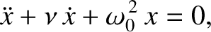
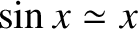
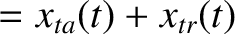
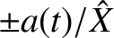
There are a number of interesting cases that are worth discussing. Consider,
first, the situation in which the driving frequency is equal to the resonant frequency; that is,
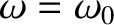 . In this case, Equation (2.87) reduces to
 |
(2.88) |
 . Thus, the driven response oscillates at the
resonant frequency,
. Thus, the driven response oscillates at the
resonant frequency,  , because both the time asymptotic and transient solutions
oscillate at this frequency. However, the amplitude of the
oscillation grows monotonically as
, because both the time asymptotic and transient solutions
oscillate at this frequency. However, the amplitude of the
oscillation grows monotonically as
 , and
so takes a time of order
, and
so takes a time of order
 (i.e., a time of order
  oscillation periods) to attain its final value
 , which
is, of course, larger that the driving amplitude by the resonant amplification
factor (or quality factor), . This behavior is illustrated in Figure 2.7.
, which
is, of course, larger that the driving amplitude by the resonant amplification
factor (or quality factor), . This behavior is illustrated in Figure 2.7.
![\includegraphics[width=0.8\textwidth]{Chapter02/fig2_08.eps}](img617.png) |
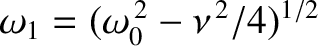
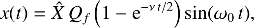
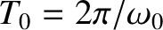
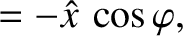
Consider the situation in which there is no damping, so that  . In this
case, Equation (2.87) yields
. In this
case, Equation (2.87) yields
![$\cos a - \cos b \equiv -2\,\sin[(a+b)/2]\,\sin[(a-b)/2]$](img620.png) . (See Appendix B.) It can be seen that the driven response oscillates relatively rapidly at the “sum frequency”
. (See Appendix B.) It can be seen that the driven response oscillates relatively rapidly at the “sum frequency”
 with an amplitude
![$a(t) = \hat{X}\,[\omega_0/(\omega_0-\omega)]\,\sin[(\omega_0-\omega)/t]$](img622.png) that modulates relatively slowly at the
“difference frequency”
that modulates relatively slowly at the
“difference frequency”
 . (Recall, that we are assuming that
is close to .) This behavior is illustrated in
Figure 2.8. The amplitude modulations shown
in Figure 2.8 are called beats, and are produced whenever two
sinusoidal oscillations of similar amplitude, and slightly different frequency,
are superposed. In this case, the two oscillations are the time asymptotic solution,
which oscillates at the driving frequency, , and the transient
solution, which oscillates at the resonant frequency, . The beats
modulate at the difference frequency,
. In the limit
. (Recall, that we are assuming that
is close to .) This behavior is illustrated in
Figure 2.8. The amplitude modulations shown
in Figure 2.8 are called beats, and are produced whenever two
sinusoidal oscillations of similar amplitude, and slightly different frequency,
are superposed. In this case, the two oscillations are the time asymptotic solution,
which oscillates at the driving frequency, , and the transient
solution, which oscillates at the resonant frequency, . The beats
modulate at the difference frequency,
. In the limit
 , Equation (2.89) yields
 |
(2.90) |
 when
when 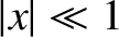 . (See Appendix B.) Thus, the resonant response of a
driven undamped oscillator is an oscillation at the resonant frequency whose
amplitude,
. (See Appendix B.) Thus, the resonant response of a
driven undamped oscillator is an oscillation at the resonant frequency whose
amplitude,
 , increases linearly in time. In this case, the period of the beats has
effectively become infinite.
, increases linearly in time. In this case, the period of the beats has
effectively become infinite.
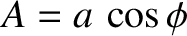
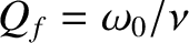
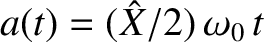
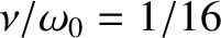
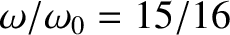
Finally, Figure 2.9 illustrates the non-resonant response of a driven damped harmonic oscillator, obtained from Equation (2.87). It can be seen that the driven response grows, showing some initial evidence of beat modulation, but eventually settles down to a steady pattern of oscillation. This behavior occurs because the transient solution, which is needed to produce beats, initially grows, but then damps away, leaving behind the constant amplitude time asymptotic solution.


![$\displaystyle = -\hat{x}\left[\frac{\omega\,\sin\varphi + (\nu/2)\,\cos\varphi}{\omega_1}\right].$](img605.png)
![$\displaystyle \simeq \hat{X}\left[\frac{2\,\omega_0\,(\omega_0-\omega)}{4\,(\om...
...\,2}}\right]\left[\cos(\omega\,t)-{\rm e}^{-\nu\,t/2}\,\cos(\omega_0\,t)\right]$](img610.png)
![$\displaystyle ~~+ \hat{X}\left[\frac{\omega_0\,\nu}{4\,(\omega_0-\omega)^{\,2}+...
...,2}}\right]\left[\sin(\omega\,t)-{\rm e}^{-\nu\,t/2}\,\sin(\omega_0\,t)\right].$](img611.png)
![$\displaystyle x(t) = \hat{X}\,\left(\frac{\omega_0}{\omega_0-\omega}\right)\sin...
...omega_0-\omega)\,t}{2}\right]\,\sin\left[\frac{(\omega_0+\omega)\,t}{2}\right],$](img619.png)
![\includegraphics[width=0.8\textwidth]{Chapter02/fig2_09.eps}](img629.png)