Magnetic Induction

Consider a one-turn loop of conducting wire $C$ which is placed in a magnetic field ${\bf B}$. The magnetic flux ${\mit\Phi}_B$ linking loop $C$ can be written

$${\mit\Phi}_B = \int_S {\bf B}\cdot d{\bf S}$$ (197)

where $S$ is any surface attached to the loop.

Suppose that the magnetic field changes in time, causing the magnetic flux ${\mit\Phi}_B$ linking circuit $C$ to vary. Let the flux change by an amount $d{\mit\Phi}_B$ in the time interval $dt$. According to Faraday's law, the emf ${\cal E}$ induced around loop $C$ is given by

$${\cal E} = -\frac{d{\mit\Phi}_B}{dt}.$$ (198)

If ${\cal E}$ is positive then the emf acts around the loop in the same sense as that indicated by the fingers of a right-hand, when the thumb points in the direction of the mean magnetic field passing through the loop. Likewise, if ${\cal E}$ is negative then the emf acts around the loop in the opposite sense to that indicated by the fingers of a right-hand, when the thumb points in the direction of the mean magnetic field passing through the loop. In the former case, we say that the emf acts in the positive direction, whereas in the latter case we say it acts in the negative direction.

Suppose that ${\cal E}>0$, so that the emf acts in the positive direction. How, exactly, is this emf produced? In order to answer this question, we need to remind ourselves what an emf actually is. When we say that an emf ${\cal E}$ acts around the loop $C$ in the positive direction, what we really mean is that a charge $q$ which circulates once around the loop in the positive direction acquires the energy $q\,{\cal E}$. How does the charge acquire this energy? Clearly, either an electric field or a magnetic field, or some combination of the two, must perform the work $q\,{\cal E}$ on the charge as it circulates around the loop. However, we have already seen, from Sect. 8.4, that a magnetic field is unable to do work on a charged particle. Thus, the charge must acquire the energy $q\,{\cal E}$ from an electric field as it circulates once around the loop in the positive direction.

According to Sect. 5, the work that the electric field does on the charge as it goes around the loop is

$$W=q\,\oint_C {\bf E}\cdot d{\bf r},$$ (199)

where $d{\bf r}$ is a line element of the loop. Hence, by energy conservation, we can write $W = q\,{\cal E}$, or

$${\cal E} = \oint_C {\bf E} \cdot d{\bf r}.$$ (200)

The term on the right-hand side of the above expression can be recognized as the line integral of the electric field around loop $C$ in the positive direction. Thus, the emf generated around the circuit $C$ in the positive direction is equal to the line integral of the electric field around the circuit in the same direction.

Equations (198) and (200) can be combined to give

$$\oint_C {\bf E} \cdot d{\bf r}= -\frac{d{\mit\Phi}_B}{dt}.$$ (201)

Thus, Faraday's law implies that the line integral of the electric field around circuit $C$ (in the positive direction) is equal to minus the time rate of change of the magnetic flux linking this circuit. Does this law just apply to conducting circuits, or can we apply it to an arbitrary closed loop in space? Well, the difference between a conducting circuit and an arbitrary closed loop is that electric current can flow around a circuit, whereas current cannot, in general, flow around an arbitrary loop. In fact, the emf ${\cal E}$ induced around a conducting circuit drives a current $I={\cal E}/R$ around that circuit, where $R$ is the resistance of the circuit. However, we can make this resistance arbitrarily large without invalidating Eq. (201). In the limit in which $R$ tends to infinity, no current flows around the circuit, so the circuit becomes indistinguishable from an arbitrary loop. Since we can place such a circuit anywhere in space, and Eq. (201) still holds, we are forced to the conclusion that Eq. (201) is valid for any closed loop in space, and not just for conducting circuits.

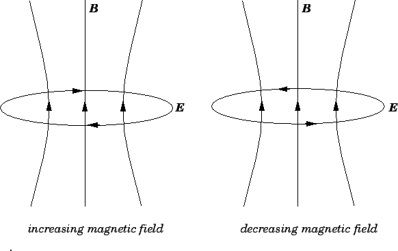
Equation (201) describes how a time-varying magnetic field generates an electric field which fills space. The strength of the electric field is directly proportional to the rate of change of the magnetic field. The field-lines associated with this electric field form loops in the plane perpendicular to the magnetic field. If the magnetic field is increasing then the electric field-lines circulate in the opposite sense to the fingers of a right-hand, when the thumb points in the direction of the field. If the magnetic field is decreasing then the electric field-lines circulate in the same sense as the fingers of a right-hand, when the thumb points in the direction of the field. This is illustrated in Fig. 35.

Figure 35: Inductively generated electric fields

We can now appreciate that when a conducting circuit is placed in a time-varying magnetic field, it is the electric field induced by the changing magnetic field which gives rise to the emf around the circuit. If the loop has a finite resistance then this electric field also drives a current around the circuit. Note, however, that the electric field is generated irrespective of the presence of a conducting circuit. The electric field generated by a time-varying magnetic field is quite different in nature to that generated by a set of stationary electric charges. In the latter case, the electric field-lines begin on positive charges, end on negative charges, and never form closed loops in free space. In the former case, the electric field-lines never begin or end, and always form closed loops in free space. In fact, the electric field-lines generated by magnetic induction behave in much the same manner as magnetic field-lines. Recall, from Sect. 5.1, that an electric field generated by fixed charges is unable to do net work on a charge which circulates in a closed loop. On the other hand, an electric field generated by magnetic induction certainly can do work on a charge which circulates in a closed loop. This is basically how a current is induced in a conducting loop placed in a time-varying magnetic field. One consequence of this fact is that the work done in slowly moving a charge between two points in an inductive electric field does depend on the path taken between the two points. It follows that we cannot calculate a unique potential difference between two points in an inductive electric field. In fact, the whole idea of electric potential breaks down in a such a field (fortunately, there is a way of salvaging the idea of electric potential in an inductive field, but this topic lies beyond the scope of this course). Note, however, that it is still possible to calculate a unique value for the emf generated around a conducting circuit by an inductive electric field, because, in this case, the path taken by electric charges is uniquely specified: i.e., the charges have to follow the circuit.