


Next: Bose-Einstein Statistics
Up: Quantum Statistics
Previous: Fermi-Dirac Statistics
Up to now, we have assumed that the number of particles,  , contained
in a given system is a fixed
number. This is a reasonable assumption if the particles possess non-zero
mass, because we are not generally considering
relativistic systems in this course (i.e., we are assuming that the particle energies are much less than their rest-mass energies).
However, this assumption breaks down for the case of photons, which are
zero-mass bosons. In fact, photons enclosed in a container
of volume
, contained
in a given system is a fixed
number. This is a reasonable assumption if the particles possess non-zero
mass, because we are not generally considering
relativistic systems in this course (i.e., we are assuming that the particle energies are much less than their rest-mass energies).
However, this assumption breaks down for the case of photons, which are
zero-mass bosons. In fact, photons enclosed in a container
of volume  , maintained at temperature
  , can readily be absorbed
or emitted by the walls. Thus, for the special case of a gas of
photons, there is no requirement that limits the total number of particles.
, can readily be absorbed
or emitted by the walls. Thus, for the special case of a gas of
photons, there is no requirement that limits the total number of particles.
It follows, from the previous discussion, that photons obey a simplified
form of Bose-Einstein statistics in which there is an unspecified
total number of particles. This type of statistics is called photon
statistics.
Consider the expression (8.21). For the case of photons, the
numbers
 assume all values
 for each
  ,
without any further restriction. It follows that the sums
,
without any further restriction. It follows that the sums
 in the
numerator and denominator are identical and, therefore, cancel. Hence,
Equation (8.21) reduces to
in the
numerator and denominator are identical and, therefore, cancel. Hence,
Equation (8.21) reduces to
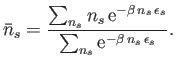 |
(8.35) |
However, the previous expression can be rewritten
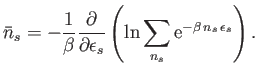 |
(8.36) |
Now, the sum on the right-hand side of the previous equation is an infinite
geometric series, which can easily be evaluated. In fact,
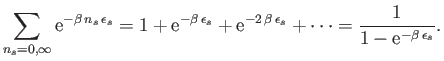 |
(8.37) |
(See Exercise 1.)
Thus, Equation (8.36) gives
 |
(8.38) |
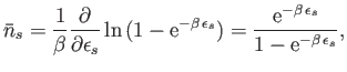
or
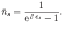 |
(8.39) |
This is known as the Planck distribution, after the German physicist
Max Planck who first proposed it in 1900 on purely empirical grounds.
Equation (8.20) can be integrated to
give
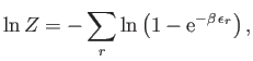 |
(8.40) |
where use has been made of Equation (8.39).
Next: Bose-Einstein Statistics
Up: Quantum Statistics
Previous: Fermi-Dirac Statistics
Richard Fitzpatrick
2016-01-25