


Next: Heat and Work
Up: Statistical Mechanics
Previous: Behavior of Density of
- Consider a particle of mass
 confined within a cubic box of dimensions
 . According to elementary quantum mechanics, the possible energy levels of this particle are given by
where  ,
,  , and
, and  are positive integers. (See Section C.10.)
- Suppose that the particle is in a given state specified by
particular values of the three quantum numbers,
,
,
. By
considering how the energy of this state must change when the length,
 , of
the box parallel to the
, of
the box parallel to the  -axis is very slowly changed by a small amount
  , show that the force exerted
by a particle in this state on a wall perpendicular to the
-axis is given
by
, show that the force exerted
by a particle in this state on a wall perpendicular to the
-axis is given
by
 .
.
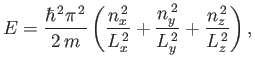
- Explicitly calculate the force per unit area (or pressure) acting on this wall.
By averaging over all possible states, find an expression for the mean pressure
on this wall. (Hint: exploit the fact that
 must all be equal, by symmetry.) Show that this mean pressure can be
written
must all be equal, by symmetry.) Show that this mean pressure can be
written
where
 is the mean energy of the particle,
and
is the mean energy of the particle,
and
 the volume of the box.
- The state of a system with
 degrees of freedom at time
  is specified by its generalized coordinates,
 , and
conjugate momenta,
, and
conjugate momenta,
 . These evolve according to
Hamilton's equations (see Section B.9):
. These evolve according to
Hamilton's equations (see Section B.9):
Here,
 is the Hamiltonian of the system.
Consider a statistical ensemble of such systems. Let
is the Hamiltonian of the system.
Consider a statistical ensemble of such systems. Let
 be the number density of systems in
phase-space. In other words, let
be the number density of systems in
phase-space. In other words, let
 be the number of states with
  lying between
and
lying between
and  ,
,  lying
between
and
lying
between
and  , et cetera, at time
.
, et cetera, at time
.
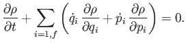
- Show that
 evolves in time according to Liouville's theorem:
[Hint: Consider how the the flux of systems into a small volume of phase-space causes the
number of systems in the volume to change in time.]
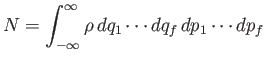
- By definition,
is the total number of systems in the ensemble. The integral is over all of
phase-space. Show that Liouville's theorem conserves the total number of systems
(i.e.,  ). You may assume that
becomes negligibly
small if any of its arguments (i.e.,
and
) becomes very large. This is equivalent to assuming that
all of the systems are localized to some region of phase-space.
). You may assume that
becomes negligibly
small if any of its arguments (i.e.,
and
) becomes very large. This is equivalent to assuming that
all of the systems are localized to some region of phase-space.
- Suppose that
 has no explicit time dependence
(i.e.,
has no explicit time dependence
(i.e.,
 ).
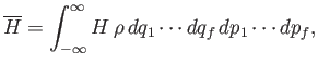
Show that the ensemble-averaged energy,
).
Show that the ensemble-averaged energy,
is a constant of the motion.
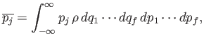
- Show that if
is also not an explicit function of the coordinate
 then the ensemble average of the conjugate momentum,
is a constant of the motion.
- Consider a system consisting of very many particles. Suppose that an
observation of a macroscopic variable,
, can result in any one of a great
many closely-spaced values,
 .
Let the (approximately constant)
spacing between adjacent values be
.
Let the (approximately constant)
spacing between adjacent values be  . The probability of occurrence of the
value
is denoted
. The probability of occurrence of the
value
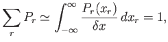
is denoted  . The probabilities are assumed to be properly
normalized, so that
. The probabilities are assumed to be properly
normalized, so that
where the summation is over all possible values. Suppose that we know the
mean and the variance of
, so that
and
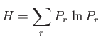
are both fixed. According to the
-theorem, the system will naturally
evolve towards a final equilibrium
state in which the quantity
is minimized. Used the method of Lagrange multipliers to minimixe
with respect to the
, subject to the constraints
that the probabilities remain properly normalized, and that the mean and variance
of
remain constant. (See Section B.6.) Show that the most general form for the
which
can achieve this goal is
This result demonstrates that the system will naturally evolve towards a final
equilibrium state
in which all of its macroscopic variables have Gaussian probability distributions,
which is in accordance with
the central limit theorem. (See Section 2.10.)
Next: Heat and Work
Up: Statistical Mechanics
Previous: Behavior of Density of
Richard Fitzpatrick
2016-01-25


![$\displaystyle P_r (x_r)\simeq \frac{\delta x}{ \sqrt{2\pi \overline{({\mit \De...
...\frac{(x_r-\overline{x})^{ 2}}{2 \overline{({\mit \Delta} x)^{ 2}}}\right].
$](img453.png)