Next: Probability Interpretation of Wavefunction
Up: Wave Mechanics
Previous: Representation of Waves via
Schrödinger's Equation
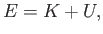
The basic premise of wave mechanics is that a massive particle of energy  and linear momentum
  , moving in the
  -direction (say),
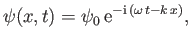
can be represented by a one-dimensional complex wavefunction of the form
-direction (say),
can be represented by a one-dimensional complex wavefunction of the form
 |
(C.15) |
where the complex amplitude,  , is arbitrary, while the wavenumber,
  , and the angular frequency,
  ,
are related to the particle momentum,
, and energy,
, via the fundamental
relations (C.3) and (C.1), respectively. The previous one-dimensional wavefunction is the solution of
a one-dimensional wave equation that determines how the wavefunction evolves in time.
As described in the following, we can guess the form of this wave equation by drawing an analogy with classical physics.
,
are related to the particle momentum,
, and energy,
, via the fundamental
relations (C.3) and (C.1), respectively. The previous one-dimensional wavefunction is the solution of
a one-dimensional wave equation that determines how the wavefunction evolves in time.
As described in the following, we can guess the form of this wave equation by drawing an analogy with classical physics.
A classical particle of mass  , moving in a one-dimensional potential
  , satisfies the energy conservation
equation
, satisfies the energy conservation
equation
 |
(C.16) |
where
 |
(C.17) |
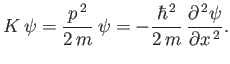
is the particle's kinetic energy. Hence,
 |
(C.18) |
is a valid, but not obviously useful, wave equation.
However, it follows from Equations (C.1) and (C.15) that
 |
(C.19) |
which can be rearranged to give
 |
(C.20) |
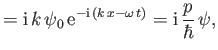
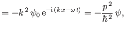
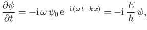
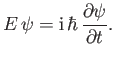
Likewise, from Equations (C.3) and (C.15),
which can be rearranged to give
 |
(C.23) |
Thus, combining Equations (C.18), (C.20), and (C.23), we obtain
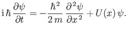 |
(C.24) |
This equation, which is known as Schrödinger's equation--because it was first formulated by Erwin Schrödinder in 1926--is the fundamental equation of wave mechanics.
For a massive particle moving in free space (i.e.,  ), the complex wavefunction (C.15) is a
solution of Schrödinger's equation, (C.24), provided
), the complex wavefunction (C.15) is a
solution of Schrödinger's equation, (C.24), provided
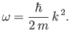 |
(C.25) |
The previous expression can be thought of as the dispersion relation for matter waves in free space. The
associated phase velocity is
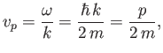 |
(C.26) |
where use has been made of Equation (C.3). However, this phase velocity is only half the classical velocity,  ,
of a massive (non-relativistic) particle.
,
of a massive (non-relativistic) particle.
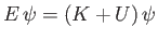
Incidentally, Equation (C.21) suggests that
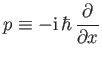 |
(C.27) |
in quantum mechanics, whereas Equation (C.24) suggests that the most general form of Schrödinger's equation is
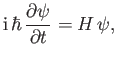 |
(C.28) |
where
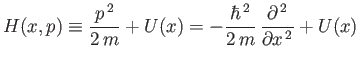 |
(C.29) |
is the Hamiltonian of the system. (See Section B.9.)
Next: Probability Interpretation of Wavefunction
Up: Wave Mechanics
Previous: Representation of Waves via
Richard Fitzpatrick
2016-01-25