Next: Equilibrium Between Phases
Up: Multi-Phase Systems
Previous: Equilibrium of Constant-Temperature Constant-Pressure
Stability of Single-Phase Substance
Consider a system in a single phase (e.g., a liquid or a solid). Let us focus attention on a small, but
macroscopic part,  , of this system. Here,
consists of a fixed number of particles,
, of this system. Here,
consists of a fixed number of particles,  . The remainder of the system is,
relatively, very large, and, therefore, acts like a reservoir held at some constant temperature,
. The remainder of the system is,
relatively, very large, and, therefore, acts like a reservoir held at some constant temperature,  , and constant pressure,
  .
According to Equation (9.25), the condition for stable equilibrium, applied to
, is
.
According to Equation (9.25), the condition for stable equilibrium, applied to
, is
 |
(9.30) |
Let the temperature,  , and the volume,
  , be the two independent parameters that specify the
macrostate of
. Consider, first, a situation where
is fixed, but
is allowed to vary. Suppose that the minimum of
, be the two independent parameters that specify the
macrostate of
. Consider, first, a situation where
is fixed, but
is allowed to vary. Suppose that the minimum of  occurs for
 , when
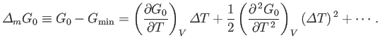
 . Expanding
about its minimum, and writing
. Expanding
about its minimum, and writing
 , we obtain
 |
(9.31) |
Here, all derivatives are evaluated at
. Because
is a stationary point (i.e., a maximum or a minimum),
 to first order in
 .
In other words,
.
In other words,
Furthermore, because  is a minimum, rather than a maximum,
 to second order in
. In other words,
to second order in
. In other words,
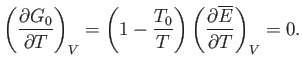
According to Equation (9.30), the condition, (9.32), that
be stationary yields
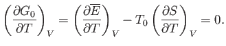 |
(9.34) |
However, the fundamental thermodynamic relation
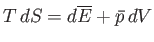 |
(9.35) |
implies that if
is fixed then
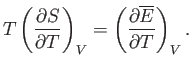 |
(9.36) |
Thus, Equation (9.34) becomes
 |
(9.37) |
Recalling that the derivatives are evaluated at
, we get
 |
(9.38) |
Thus, we arrive at the rather obvious conclusion that a necessary condition for equilibrium is that the temperature of the subsystem
be the same as
that of the surrounding medium.
Equations (9.33) and (9.37) imply that
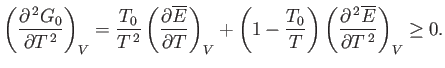 |
(9.39) |
Recalling that the derivatives are evaluated at
, and that
 , the second term on the right-hand side of
the previous equation vanishes, and we obtain
, the second term on the right-hand side of
the previous equation vanishes, and we obtain
 |
(9.40) |
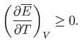
However, this derivative is simply the heat capacity,  , at constant volume. Thus, we deduce that a fundamental
criterion for the stability of any phase is
, at constant volume. Thus, we deduce that a fundamental
criterion for the stability of any phase is
 |
(9.41) |
The previous condition is a particular example of a very general rule, known as Le Chátelier's principle, which states that
If a system is in a stable equilibrium then any spontaneous change of its parameters must give rise to processes that tend to
restore the system to equilibrium.
To show how this principle applies to the present case, suppose that the temperature,
, of the subsystem
has increased
above that of its surroundings,  , as a result of a spontaneous fluctuation. The process brought into play is the spontaneous flow of heat
from system
, at the higher temperature, to its surroundings
, which brings about a decrease in the energy,
, as a result of a spontaneous fluctuation. The process brought into play is the spontaneous flow of heat
from system
, at the higher temperature, to its surroundings
, which brings about a decrease in the energy,
 , of
(i.e.,
, of
(i.e.,
 ). By Le Chátelier's principle, this energy decrease must act to decrease the temperature of
(i.e.,
). By Le Chátelier's principle, this energy decrease must act to decrease the temperature of
(i.e.,
 ), so as to restore
to its equilibrium state (in which its temperature is the same as its surroundings). Hence, it follows that
), so as to restore
to its equilibrium state (in which its temperature is the same as its surroundings). Hence, it follows that
 and
have the same sign, so
that
and
have the same sign, so
that
 , in agreement with Equation (9.40).
Suppose, now, that the temperature of subsystem
is fixed at  , but that its volume,
, is allowed to
vary. We can write
, but that its volume,
, is allowed to
vary. We can write
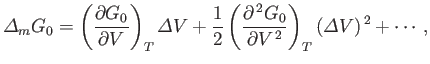 |
(9.42) |
where
 , and the expansion is about the volume
 at which
attains its
minimum value. The condition that
is stationary yields
at which
attains its
minimum value. The condition that
is stationary yields
 |
(9.43) |
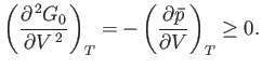
The condition that the stationary point is a minimum gives
 |
(9.44) |
Making use of Equation (9.30), we get
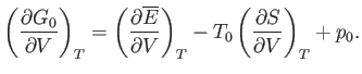 |
(9.45) |
However, Equation (9.35) implies that
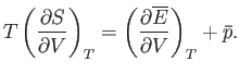 |
(9.46) |
Hence,
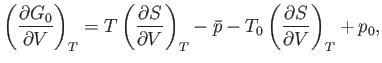 |
(9.47) |
or
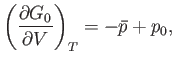 |
(9.48) |
because
. Thus, the condition (9.43) yields
 |
(9.49) |
This rather obvious result states that in equilibrium the pressure of subsystem
must be equal to that of the surrounding medium.
Equations (9.44) and (9.48) imply that
 |
(9.50) |
When expressed in terms of the isothermal compressibility,
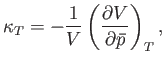 |
(9.51) |
the stability criterion (9.50) is equivalent to
 |
(9.52) |
To show how the preceding stability condition is consistent with Le Chátelier's principle, suppose that the volume of subsystem
has increased by an amount
 , as a result of a spontaneous fluctuation. The pressure,
  , of
must then
decrease below that of its surroundings (i.e.,
, of
must then
decrease below that of its surroundings (i.e.,
 ) in order to ensure that the net force exerted on
by
its surroundings is such as to reduce the volume of
back towards its equilibrium value. In other words,
) in order to ensure that the net force exerted on
by
its surroundings is such as to reduce the volume of
back towards its equilibrium value. In other words,
 and
and
 must have opposite signs, implying that
 .
.
The preceding discussion allows us to characterize the spontaneous volume fluctuations of the small subsystem
. The
most probable situation is that where
takes the value  that minimizes
, so that
that minimizes
, so that
 .
Let
.
Let  denote the probability that the volume of
lies between
and
denote the probability that the volume of
lies between
and  . According to Equation (9.29),
![$\displaystyle P(V) dV \propto \exp\left[-\frac{G_0(V)}{k T_0}\right] dV.$](img2697.png) |
(9.53) |
However, when
is small, the expansion (9.42) is applicable. By virtue of Equations (9.43), (9.50),
and (9.51), the expansion yields
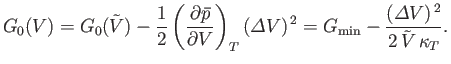 |
(9.54) |
Thus, Equation (9.53) becomes
![$\displaystyle P(V) dV =B\exp\left[-\frac{(V-\tilde{V})^{ 2}}{2 k T_0 \kappa_T \tilde{V}}\right]dV,$](img2699.png) |
(9.55) |
where we have absorbed
 into the constant of proportionality,
  . Of course,
can be determined via the requirement that
the integral of
over all possible values of the volume,
, be equal to unity.
. Of course,
can be determined via the requirement that
the integral of
over all possible values of the volume,
, be equal to unity.
The probability distribution (9.55) is a Gaussian whose maximum lies at
. Thus,
is equal to the
mean volume,
 . Moreover, the standard deviation of the spontaneous fluctuations of
about its mean value is
. Moreover, the standard deviation of the spontaneous fluctuations of
about its mean value is
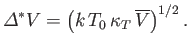 |
(9.56) |
(See Section 2.9.)
The fluctuations in
imply corresponding fluctuations in the number of particles per unit volume,  , (and, hence, in the mean
density) of the subsystem
. The fluctuations in
, (and, hence, in the mean
density) of the subsystem
. The fluctuations in  are centered on the mean value
 . For relatively
small fluctuations,
. For relatively
small fluctuations,
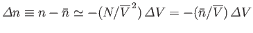 .
Hence,
.
Hence,
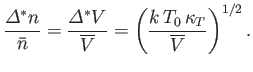 |
(9.57) |
Note that the relative magnitudes of the density and volume fluctuations are inversely proportional to the
square-root of the volume,
, under consideration.
An interesting situation arises when
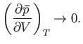 |
(9.58) |
In this limit,
 , and the density fluctuations become very large. [They do not, however, become infinite,
because the neglect of third-order, and higher, terms in the expansion (9.42) is no longer justified.]
The condition
, and the density fluctuations become very large. [They do not, however, become infinite,
because the neglect of third-order, and higher, terms in the expansion (9.42) is no longer justified.]
The condition
 defines the so-called critical point of the substance, at which the
distinction between its liquid and gas phases disappears. (See Section 9.10.) The very large density fluctuations at the critical
point lead to strong scattering of light. As a result, a substance that is ordinarily transparent will assume a milky-white
appearance at its critical point (e.g.,
defines the so-called critical point of the substance, at which the
distinction between its liquid and gas phases disappears. (See Section 9.10.) The very large density fluctuations at the critical
point lead to strong scattering of light. As a result, a substance that is ordinarily transparent will assume a milky-white
appearance at its critical point (e.g.,
 when it approaches its critical point at 304K and 73 atmospheres). This interesting
phenomenon is called critical-point opalecance.
when it approaches its critical point at 304K and 73 atmospheres). This interesting
phenomenon is called critical-point opalecance.
Next: Equilibrium Between Phases
Up: Multi-Phase Systems
Previous: Equilibrium of Constant-Temperature Constant-Pressure
Richard Fitzpatrick
2016-01-25