


Next: Harmonic Perturbations
Up: Time-Dependent Perturbation Theory
Previous: Spin Magnetic Resonance
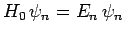
Let us recall the analysis of Sect. 13.2. The  are the stationary orthonormal eigenstates of the time-independent
unperturbed Hamiltonian,
are the stationary orthonormal eigenstates of the time-independent
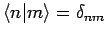
unperturbed Hamiltonian,  . Thus,
 ,
where the
,
where the  are the unperturbed energy levels, and
 . Now, in the presence of a small
time-dependent perturbation to the Hamiltonian,
. Now, in the presence of a small
time-dependent perturbation to the Hamiltonian,  , the wavefunction
of the system takes the form
, the wavefunction
of the system takes the form
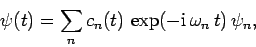 |
(1057) |
where
 . The amplitudes
  satisfy
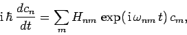 |
(1058) |
where
 and
and
 . Finally, the probability of finding the system in the
  th eigenstate
at time
th eigenstate
at time  is simply
 |
(1059) |
(assuing that, initially,
 ).
).
Suppose that at  the system is in some initial energy eigenstate labeled
  . Equation (1058) is, thus, subject to the initial condition
 |
(1060) |
Let us attempt a perturbative solution of Eq. (1058) using
the ratio of  to (or
  to
to
 , to be more exact) as our expansion parameter.
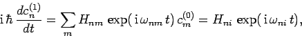
Now, according to (1058), the
, to be more exact) as our expansion parameter.
Now, according to (1058), the  are constant in time in the
absence of the perturbation. Hence, the zeroth-order solution is simply
are constant in time in the
absence of the perturbation. Hence, the zeroth-order solution is simply
 |
(1061) |
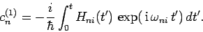
The first-order solution is obtained, via iteration, by substituting the zeroth-order
solution into the right-hand side of Eq. (1058). Thus, we obtain
 |
(1062) |
subject to the boundary condition
 . The solution to
the above equation is
. The solution to
the above equation is
 |
(1063) |
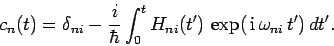
It follows that, up to first-order in our perturbation expansion,
 |
(1064) |
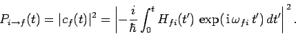
Hence, the probability of finding the system in some final energy
eigenstate labeled  at time , given that it is definitely in a different initial energy eigenstate labeled at time , is
 |
(1065) |
Note, finally, that our perturbative solution is clearly only valid provided
 |
(1066) |
Next: Harmonic Perturbations
Up: Time-Dependent Perturbation Theory
Previous: Spin Magnetic Resonance
Richard Fitzpatrick
2010-07-20