Next: Simple Harmonic Oscillator
Up: One-Dimensional Potentials
Previous: Alpha Decay
Consider a particle of mass  and energy
  interacting with the
simple square potential well
interacting with the
simple square potential well
![\begin{displaymath}
V(x) = \left\{\begin{array}{lcl}
-V_0&\mbox{\hspace{1cm}}&\m...
... x\leq a/2$}\ [0.5ex]
0&&\mbox{otherwise}
\end{array}\right.,
\end{displaymath}](img952.png) |
(372) |
where  .
.
Now, if  then the particle is unbounded. Thus, when the particle encounters the well
it is either reflected or transmitted. As is easily demonstrated, the reflection and transmission
probabilities are given by Eqs. (327) and (328), respectively,
where
then the particle is unbounded. Thus, when the particle encounters the well
it is either reflected or transmitted. As is easily demonstrated, the reflection and transmission
probabilities are given by Eqs. (327) and (328), respectively,
where
Suppose, however, that  . In this case, the particle
is bounded (i.e.,
. In this case, the particle
is bounded (i.e.,
 as
as
 ).
Is is possible to find bounded solutions of Schrödinger's equation
in the finite square potential well (372)?
).
Is is possible to find bounded solutions of Schrödinger's equation
in the finite square potential well (372)?
Now, it is easily seen that independent solutions of Schrödinger's equation (301)
in the symmetric [i.e.,  ] potential (372)
must be either totally symmetric [i.e.,
] potential (372)
must be either totally symmetric [i.e.,
 ], or
totally anti-symmetric [i.e.,
], or
totally anti-symmetric [i.e.,
 ]. Moreover,
the solutions must satisfy the boundary condition
]. Moreover,
the solutions must satisfy the boundary condition
 |
(375) |
Let us, first of all, search for a totally symmetric solution.
In the region to the left of the well (i.e.  ), the
solution of Schrödinger's equation which satisfies the
boundary condition
), the
solution of Schrödinger's equation which satisfies the
boundary condition
 and
and
 is
is
 |
(376) |
where
 |
(377) |
By symmetry, the solution in the region to the right of the well (i.e.,
 ) is
) is
 |
(378) |
The solution inside the well (i.e.,  ) which
satisfies the symmetry constraint
is
) which
satisfies the symmetry constraint
is
 |
(379) |
where
 |
(380) |
Here, we have assumed that  .
The constraint that
.
The constraint that  and its first derivative be continuous at the
edges of the well (i.e., at
and its first derivative be continuous at the
edges of the well (i.e., at  ) yields
 |
(381) |
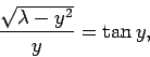
Let  . It follows that
 |
(382) |
where
 |
(383) |
Moreover, Eq. (381) becomes
 |
(384) |
with
 |
(385) |
Here,  must lie in the range
 : i.e.,
must lie in the range
: i.e.,
must lie in the range  .
.
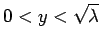
Figure:
The curves  (solid) and
 (dashed), calculated for
 . The latter curve takes the
value
. The latter curve takes the
value  when
when
 .
.
 |
Now, the solutions to Eq. (384) correspond to the
intersection of the curve
with the curve
. Figure 16 shows these two curves plotted for
a particular value of  . In this case, the curves intersect
twice, indicating the existence of two totally symmetric bound states in the well.
Moreover, it is evident, from the figure, that as increases (i.e., as the well becomes
deeper) there are more and more bound states. However, it is also evident that there is
always at least one totally symmetric bound state, no matter how small
becomes (i.e., no matter how shallow the well becomes). In the limit
. In this case, the curves intersect
twice, indicating the existence of two totally symmetric bound states in the well.
Moreover, it is evident, from the figure, that as increases (i.e., as the well becomes
deeper) there are more and more bound states. However, it is also evident that there is
always at least one totally symmetric bound state, no matter how small
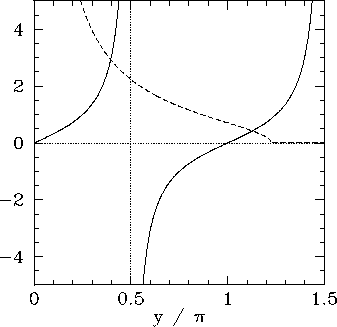
becomes (i.e., no matter how shallow the well becomes). In the limit  (i.e., the limit in which the well becomes very deep), the
solutions to Eq. (384) asymptote to the roots of
(i.e., the limit in which the well becomes very deep), the
solutions to Eq. (384) asymptote to the roots of
 .
This gives
.
This gives
 , where
  is a positive integer, or
 |
(386) |
These solutions are equivalent to the odd- infinite square well solutions
specified by Eq. (307).
infinite square well solutions
specified by Eq. (307).
Figure:
The curves (solid) and
 (dashed), calculated for
.
(dashed), calculated for
.
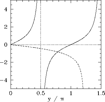 |
For the case of a totally anti-symmetric bound state, similar analysis to the
above yields
 |
(387) |
The solutions of this equation correspond to the intersection of the
curve with the curve
. Figure 17 shows these two curves plotted for
the same value of as that used in Fig. 16. In this
case, the curves intersect once, indicating the existence of
a single totally anti-symmetric bound state in the well. It is, again, evident, from the figure, that as increases (i.e., as the well becomes
deeper) there are more and more bound states. However, it is also evident that
when becomes sufficiently small [i.e.,
 ] then there is no totally
anti-symmetric bound state. In other words, a very shallow potential well
always possesses a totally symmetric bound state, but does not generally
possess a totally anti-symmetric bound state. In the limit
(i.e., the limit in which the well becomes very deep), the
solutions to Eq. (387) asymptote to the roots of
] then there is no totally
anti-symmetric bound state. In other words, a very shallow potential well
always possesses a totally symmetric bound state, but does not generally
possess a totally anti-symmetric bound state. In the limit
(i.e., the limit in which the well becomes very deep), the
solutions to Eq. (387) asymptote to the roots of  .
This gives
.
This gives  , where is a positive integer, or
 |
(388) |
These solutions are equivalent to the even- infinite square well solutions
specified by Eq. (307).
Next: Simple Harmonic Oscillator
Up: One-Dimensional Potentials
Previous: Alpha Decay
Richard Fitzpatrick
2010-07-20