


Next: Born Approximation
Up: Scattering Theory
Previous: Introduction
Consider time-independent, energy conserving scattering in which the Hamiltonian
of the system is written
 |
(1250) |
where
 |
(1251) |
is the Hamiltonian of a free particle of mass  , and
, and  the scattering potential. This potential is assumed to only be
non-zero in a fairly localized region close to the origin. Let
the scattering potential. This potential is assumed to only be
non-zero in a fairly localized region close to the origin. Let
 |
(1252) |
represent an incident beam of particles, of number density  , and
velocity
, and
velocity
 . Of course,
 |
(1253) |
where
 is the particle energy.
Schrödinger's equation for the scattering problem is
is the particle energy.
Schrödinger's equation for the scattering problem is
 |
(1254) |
subject to the boundary condition
 as
as
 .
.
The above equation can be rearranged to give
 |
(1255) |
Now,
 |
(1256) |
is known as the Helmholtz equation. The solution to this
equation is well-known:![[*]](footnote.png)
 |
(1257) |
Here,  is any solution of
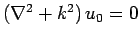 .
Hence, Eq. (1255) can be inverted, subject to the boundary condition
as
, to give
.
Hence, Eq. (1255) can be inverted, subject to the boundary condition
as
, to give
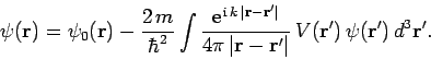 |
(1258) |
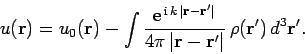
Let us calculate the value of the wavefunction  well outside the
scattering region. Now, if
well outside the
scattering region. Now, if  then
then
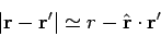 |
(1259) |
to first-order in  , where
  is a unit vector
which points from the scattering region to the observation point.
It is helpful to define
is a unit vector
which points from the scattering region to the observation point.
It is helpful to define
 . This is the wavevector
for particles with the same energy as the incoming particles (i.e.,
. This is the wavevector
for particles with the same energy as the incoming particles (i.e.,
 ) which propagate from the scattering region to the observation
point. Equation (1258) reduces to
) which propagate from the scattering region to the observation
point. Equation (1258) reduces to
![\begin{displaymath}
\psi({\bf r}) \simeq \sqrt{n}\left[{\rm e}^{ {\rm i} {\bf ...
...
+ \frac{e^{ {\rm i} k r}}{r} f({\bf k}, {\bf k}')\right],
\end{displaymath}](img2858.png) |
(1260) |
where
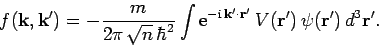 |
(1261) |
The first term on the right-hand side of Eq. (1260) represents the incident particle
beam, whereas the second term represents an outgoing spherical wave
of scattered particles.
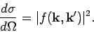
The differential scattering cross-section
 is
defined as the number of particles per unit time scattered into
an element of solid angle
is
defined as the number of particles per unit time scattered into
an element of solid angle  , divided by the incident
particle flux. From Sect. 7.2, the probability flux (i.e., the
particle flux) associated with a wavefunction
, divided by the incident
particle flux. From Sect. 7.2, the probability flux (i.e., the
particle flux) associated with a wavefunction  is
is
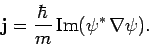 |
(1262) |
Thus, the particle flux associated with the incident wavefunction  is
is
 |
(1263) |
where
is the velocity of the incident
particles. Likewise, the particle flux associated with the scattered
wavefunction  is
is
 |
(1264) |
where
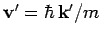 is the velocity of the scattered particles.
Now,
is the velocity of the scattered particles.
Now,
 |
(1265) |
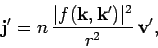
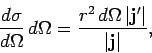
which yields
 |
(1266) |
Thus,
 gives the differential cross-section
for particles with incident velocity
to be scattered such that their final velocities are directed into a range of
solid angles about
. Note that the scattering
conserves energy, so that
gives the differential cross-section
for particles with incident velocity
to be scattered such that their final velocities are directed into a range of
solid angles about
. Note that the scattering
conserves energy, so that
 and
and
 .
.
Next: Born Approximation
Up: Scattering Theory
Previous: Introduction
Richard Fitzpatrick
2010-07-20