


Next: Exercises
Up: Time-Dependent Perturbation Theory
Previous: Electric Quadrupole Transitions
Photo-Ionization
As a final example, let us investigate the photo-ionization of atomic hydrogen. In this phenomenon, a photon of angular frequency  is absorbed by an
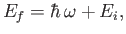
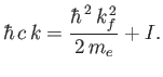
electron that occupies the ground state of a hydrogen atom. The final energy of the electron,
is absorbed by an
electron that occupies the ground state of a hydrogen atom. The final energy of the electron,
 |
(8.221) |
where  is the (negative) hydrogen ground-state energy, is assumed to be positive, which corresponds to an unbound state. In other
words, the absorption of the photon causes the hydrogen atom to dissociate.
is the (negative) hydrogen ground-state energy, is assumed to be positive, which corresponds to an unbound state. In other
words, the absorption of the photon causes the hydrogen atom to dissociate.
Let
 and
and
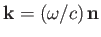
 be the wavevector and electric polarization vector of the photon, respectively. (Recall that
  and
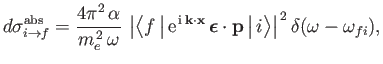
are both unit vectors.) It follows from Equations (8.136) and
(8.152) that the absorption cross-section of the hydrogen atom can be written
and
are both unit vectors.) It follows from Equations (8.136) and
(8.152) that the absorption cross-section of the hydrogen atom can be written
 |
(8.222) |
where  is the electron momentum, and
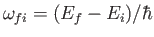 . Here, we have written
 , rather than
 , because we are only
considering final states in which the electron momentum,
, because we are only
considering final states in which the electron momentum,  , is directed into the range of solid angles
 . As discussed in Section 8.6, we must operate on the previous expression with
 , where
  is the density of final states, to obtain the true absorption cross-section, which takes the
form
is the density of final states, to obtain the true absorption cross-section, which takes the
form
 |
(8.223) |
Here, we have made use of the fact that
is an Hermitian operator, and have also employed the result
 , where
  is a constant. (See Exercise 19.)
The electron is initially in the hydrogen ground state, whose wavefunction takes the form
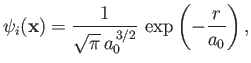 |
(8.224) |
where  is the Bohr radius. (See Chapter 4.) On the other hand, the final
electron state is assumed to be a plane-wave state whose wavefunction is
is the Bohr radius. (See Chapter 4.) On the other hand, the final
electron state is assumed to be a plane-wave state whose wavefunction is
 |
(8.225) |
In writing this expression, we have conveniently assumed that the emitted electron is contained in a cubic
box of dimension  , and volume
  . Furthermore, the electron wavefunction is required to be periodic at the
boundaries of the box. Of course, we can later take the limit
. Furthermore, the electron wavefunction is required to be periodic at the
boundaries of the box. Of course, we can later take the limit
 to obtain the general case. (However,
it turns out that this is not necessary, because the final result does not depend on
to obtain the general case. (However,
it turns out that this is not necessary, because the final result does not depend on  , provided that
.) The
wavefunction of the final electron state is normalized such that the probability of finding the electron in the box is unity:
that is,
, provided that
.) The
wavefunction of the final electron state is normalized such that the probability of finding the electron in the box is unity:
that is,
 |
(8.226) |
Note that the final state is an eigenstate of
belonging to the eigenvalue
 |
(8.227) |
(This follows from the standard Schrödinger representation
 .) Furthermore, in writing the
wavefunction (8.228), we have neglected any interaction between the emitted electron and the hydrogen
nucleus. This neglect is only reasonable provided the final electron energy,
.) Furthermore, in writing the
wavefunction (8.228), we have neglected any interaction between the emitted electron and the hydrogen
nucleus. This neglect is only reasonable provided the final electron energy,
 |
(8.228) |
is much larger than the ionization energy (i.e., the binding energy) of the hydrogen atom,
 |
(8.229) |
The condition  yields
 |
(8.230) |
In other words, the de Broglie wavelength of the emitted electron must be much larger than the typical dimension of the
hydrogen atom.
Let us calculate
. Suppose that
 . The periodicity constraint on
 at the boundaries of the box imply that
where  ,
,  , and
, and  are integers. It follows that
 |
(8.234) |
where
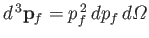
 , et cetera. Thus, the number of final electron states contained in a volume
 of momentum space is
 , where
 |
(8.235) |
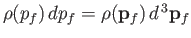
Note that
 is constant. Hence, we deduce that the number of final electron states for which
 lies between
  and
and  , and
is directed into the
range of solid angles
, is
, and
is directed into the
range of solid angles
, is
 , where
 . In other words,
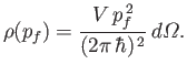 |
(8.236) |
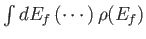
Finally, the number of final electron states whose energies lie between  and
and  is
is
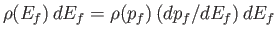 , which yields
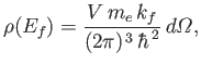 |
(8.237) |
where use has been made of Equations (8.230) and (8.231).
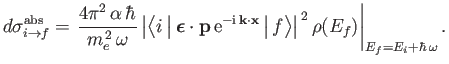
Equations (8.226) and (8.240) imply that the differential cross-section for the
photo-ionization of atomic hydrogen takes the form
 |
(8.238) |
Furthermore, making use of Equations (8.227) and (8.228), we can write
 |
(8.239) |
where
 |
(8.240) |
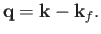
Note, by momentum conservation, that
 is the recoil momentum of the hydrogen nucleus after ionization.
The usual Schrödinger representation
is the recoil momentum of the hydrogen nucleus after ionization.
The usual Schrödinger representation
 reveals that
 |
(8.241) |
where we have made use of the standard electromagnetic result
 [49].
[49].
Assuming that
, we can write
 |
(8.242) |
where
 . Here,
  ,
,  are spherical angles whose polar axis is parallel to
  .
Thus, we obtain
.
Thus, we obtain
 |
(8.243) |
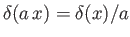
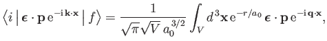
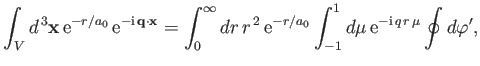
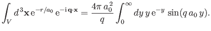
However (see Exercise 20),
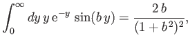 |
(8.244) |
which implies that
![$\displaystyle \int_V d^{\,3}{\bf x} \,{\rm e}^{-r/a_0}\,{\rm e}^{-{\rm i}\,{\bf q}\cdot{\bf x}}=\frac{8\pi\,a_0^{\,3}}{[1+(q\,a_0)^2]^{\,2}}.$](img2768.png) |
(8.245) |
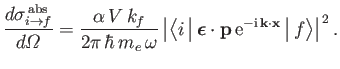
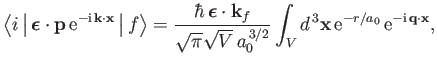
Thus, Equations (8.241), (8.244), and (8.248) yield
![$\displaystyle \frac{d\sigma_{i\rightarrow f}^{\,{\rm abs}}}{d{\mit\Omega}} =\fr...
...ox{\boldmath$\epsilon$}\cdot{\bf k}_f)^{\,2}\,a_0^{\,3}}{[1+(q\,a_0)^2]^{\,4}},$](img2769.png) |
(8.246) |
where use has been made of the standard electromagnetic dispersion relation
 [49].
[49].
It is convenient to orientate our coordinate system such that
 and
and
 .
Thus, we can specify the direction of the emitted electron in terms of the conventional
polar angles,
.
Thus, we can specify the direction of the emitted electron in terms of the conventional
polar angles,  and
and  . In fact,
 |
(8.247) |
and
 , with
 .
Hence, we obtain
.
Hence, we obtain
![$\displaystyle \frac{d\sigma_{i\rightarrow f}^{\,{\rm abs}}}{d{\mit\Omega}} =2^{...
...f\,a_0)^3\,\frac{\sin^2\theta\,\cos^2\varphi}{[1+(q\,a_0)^2]^{\,4}}\,a_0^{\,2},$](img2774.png) |
(8.248) |
where
 |
(8.249) |
is the normalized ionization energy.
Now, energy conservation demands that
 |
(8.250) |
[See Equation (8.224).] This expression can be rearranged to give
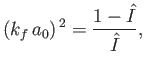 |
(8.251) |
and
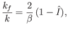 |
(8.252) |
where
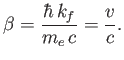 |
(8.253) |
Here,  is the speed of the emitted electron. However, we have already seen, from Equation (8.233),
that the approximations made in deriving Equation (8.251) are only
accurate when
is the speed of the emitted electron. However, we have already seen, from Equation (8.233),
that the approximations made in deriving Equation (8.251) are only
accurate when
 . Hence, according to Equation (8.254), we also
require that
. Hence, according to Equation (8.254), we also
require that
 . Furthermore, because we are working in the non-relativistic limit, we need
 .
From Equation (8.255), this necessitates
.
From Equation (8.255), this necessitates
 |
(8.254) |
Finally, the inequality
can be combined with the previous inequality to give
 |
(8.255) |
as the condition for the validity of Equation (8.251).
Now,
 |
(8.256) |
which implies that
 |
(8.257) |
where use has been made of Equation (8.255), and we have neglected terms of order
 . Equations (8.251), (8.254), and (8.260) can be combined to give the following
expression for the differential photo-ionization cross-section of atomic hydrogen:
. Equations (8.251), (8.254), and (8.260) can be combined to give the following
expression for the differential photo-ionization cross-section of atomic hydrogen:
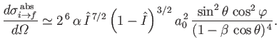 |
(8.258) |
Integrating over all solid angle, and neglecting terms of order
, the total
cross-section becomes
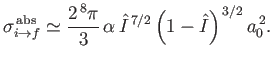 |
(8.259) |
(See Exercise 21.)
Note that the previous two expressions are only accurate in the limits
and
. Nevertheless, we
have retained the factors
 in these formulae because they emphasize that there is
a threshold photon energy for photo-ionization: namely,
in these formulae because they emphasize that there is
a threshold photon energy for photo-ionization: namely,
 . For
. For
 (i.e.,
  ), the incident photons are not energetic enough to ionize the hydrogen atom, so there
are no emitted photoelectrons. Consequently, the cross-section for photo-ionization tends to zero as
), the incident photons are not energetic enough to ionize the hydrogen atom, so there
are no emitted photoelectrons. Consequently, the cross-section for photo-ionization tends to zero as  approaches
unity from below. We have retained the factor involving
approaches
unity from below. We have retained the factor involving  in Equation (8.261) because it makes clear that
the photoelectrons are emitted preferentially in the directions
in Equation (8.261) because it makes clear that
the photoelectrons are emitted preferentially in the directions  ,
,  and
and
 .
Thus, in the non-relativistic limit,
.
Thus, in the non-relativistic limit,
 , the electrons are emitted preferentially along
the
, the electrons are emitted preferentially along
the  -axis (i.e., parallel or anti-parallel to the incident photon's electric polarization vector.) On the
other hand, as relativistic effects become important, and
consequently increases, the
directions of preferentially emission are beamed forward (i.e., they acquire a component parallel to
the wavevector of the incident photon.) An accurate expression for the photo-ionization cross-section close to
the ionization threshold (i.e.,
-axis (i.e., parallel or anti-parallel to the incident photon's electric polarization vector.) On the
other hand, as relativistic effects become important, and
consequently increases, the
directions of preferentially emission are beamed forward (i.e., they acquire a component parallel to
the wavevector of the incident photon.) An accurate expression for the photo-ionization cross-section close to
the ionization threshold (i.e.,
 ) can only be obtained using unbound positive energy hydrogen atom wavefunctions as the
final electron states [106]. Likewise, an accurate expression for the cross-section in the finite-
limit requires a relativistic treatment of the problem [96,97].
) can only be obtained using unbound positive energy hydrogen atom wavefunctions as the
final electron states [106]. Likewise, an accurate expression for the cross-section in the finite-
limit requires a relativistic treatment of the problem [96,97].
Next: Exercises
Up: Time-Dependent Perturbation Theory
Previous: Electric Quadrupole Transitions
Richard Fitzpatrick
2016-01-22


