


Next: Forbidden Transitions
Up: Time-Dependent Perturbation Theory
Previous: Spontaneous Emission of Radiation
Electric Dipole Transitions
In general, the wavelength of the type of
electromagnetic radiation that induces, or is emitted during, transitions
between different atomic states is much larger than the
typical size of
a light atom. Thus, recalling that
 , the expession
![$\displaystyle \exp\left[\,{\rm i}\left(\frac{\omega}{c}\right){\bf n}\cdot{\bf x}\right] = 1 + {\rm i}\,\frac{\omega}{c} \,{\bf n}\cdot{\bf x} + \cdots,$](img2591.png) |
(8.164) |
is well approximated by its first term, unity.
This approximation is known as the electric dipole approximation.
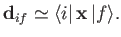
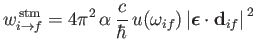
It follows from Equation (8.136) that
 |
(8.165) |
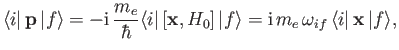
It is readily demonstrated from Equations (3.33) and (8.132) that
![$\displaystyle [{\bf x}, H_0] = \frac{{\rm i}\, \hbar \,{\bf p}}{m_e},$](img2593.png) |
(8.166) |
so
 |
(8.167) |
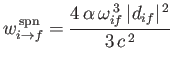
which implies that
 |
(8.168) |
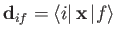
Here,
 is termed the electric dipole matrix element.
Recall from Equations (8.149), (8.150), and
(8.164) that
is termed the electric dipole matrix element.
Recall from Equations (8.149), (8.150), and
(8.164) that
 |
(8.169) |
for absorption, and
 |
(8.170) |
for stimulated emission, and with
 |
(8.171) |
for spontaneous emission.
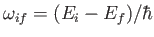
We have already seen, from Section 7.4, that
 for a hydrogen-like atom,
unless the initial and final states satisfy
for a hydrogen-like atom,
unless the initial and final states satisfy
 and
and
 .
Here,
.
Here,  is the azimuthal quantum number, and
  the magnetic quantum number. Moreover,
 is the difference between the azimuthal quantum numbers of the initial and final
states, et cetera.
It is easily demonstrated that
is the difference between the azimuthal quantum numbers of the initial and final
states, et cetera.
It is easily demonstrated that
 and
and
 are only non-zero if
,
and
are only non-zero if
,
and
 .
(See Exercise 10.)
It follows that the electric dipole matrix elements,
.
(See Exercise 10.)
It follows that the electric dipole matrix elements,
 , which control the rates
of so-called electric dipole transitions, via Equations (8.172)-(8.174), are only non-zero if
, which control the rates
of so-called electric dipole transitions, via Equations (8.172)-(8.174), are only non-zero if
Here,  is the spin quantum number, which is defined as the eigenvalue of
  divided by
  .
(Of course,
.
(Of course,
 because
  does not explicitly depend on spin.)
These expressions are termed the selection rules for electric dipole transitions. It
is clear, for instance, that the electric dipole selection rules permit
a transition from a
does not explicitly depend on spin.)
These expressions are termed the selection rules for electric dipole transitions. It
is clear, for instance, that the electric dipole selection rules permit
a transition from a  state to a
  state of a hydrogen-like atom, but disallow a transition
from a
state of a hydrogen-like atom, but disallow a transition
from a  to a
state. The latter transition is called a forbidden
transition. The previous selection rules can also be written in the
slightly more general form
to a
state. The latter transition is called a forbidden
transition. The previous selection rules can also be written in the
slightly more general form
where  and
and  are the standard quantum numbers associated with the total angular momentum, and the
projection of the total angular momentum along the
are the standard quantum numbers associated with the total angular momentum, and the
projection of the total angular momentum along the  -axis, respectively [23]. (These new rules
are evident from a perusal of the results of Exercise 15.) Note, however, that an electric
dipole transition between two
-axis, respectively [23]. (These new rules
are evident from a perusal of the results of Exercise 15.) Note, however, that an electric
dipole transition between two  states is forbidden [23].
Let us estimate the typical spontaneous emission rate for an electric dipole transition in a
hydrogen atom. We expect the matrix element
, defined in Equation (8.171), to be
of order  , where
is the Bohr radius.
We also expect
, where
is the Bohr radius.
We also expect
 to be of order
 , where
  is the hydrogen ground-state energy. It thus
follows from Equation (8.174) that
is the hydrogen ground-state energy. It thus
follows from Equation (8.174) that
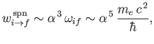 |
(8.177) |
where
 is
the fine structure constant. This is an important result, because our perturbation
expansion is based on the assumption that the transition rate between different energy
eigenstates is much less than the frequency of phase oscillation of these states. In other words,
is
the fine structure constant. This is an important result, because our perturbation
expansion is based on the assumption that the transition rate between different energy
eigenstates is much less than the frequency of phase oscillation of these states. In other words,
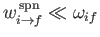 . This is indeed the
case.
. This is indeed the
case.
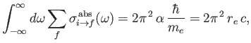
According to Equation (8.152), the absorption cross-section associated with atomic
transitions between an initial state of energy  and a final state of energy
  can be written
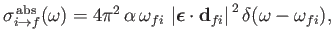 |
(8.178) |
where
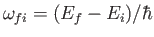 .
Suppose, for the sake of argument, that the electromagnetic radiation is polarized in the
.
Suppose, for the sake of argument, that the electromagnetic radiation is polarized in the  -direction, so that

 . According to Equation (8.181), if such radiation is incident on a hydrogen-like atom then the net absorption cross-section, summed over all final states, and integrated over
all possible angular frequencies of the radiation, can be written
. According to Equation (8.181), if such radiation is incident on a hydrogen-like atom then the net absorption cross-section, summed over all final states, and integrated over
all possible angular frequencies of the radiation, can be written
 |
(8.179) |
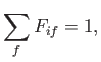
where the dimensionless parameter
 |
(8.180) |
is termed the oscillator strength associated with radiation-induced electric dipole transitions between states  and
and  .
Note that if state
is the ground state (i.e., the lowest energy state) then the sum in Equation (8.182)
is over all atomic states. On the other hand, if state
is not the ground state then the sum is restricted to
states whose energies are greater than
(because we must have
for absorption).
Now, a straightforward generalization of the result proved in Exercise 6 yields the so-called
Thomas-Reiche-Kuhn sum rule [110,70,90]:
.
Note that if state
is the ground state (i.e., the lowest energy state) then the sum in Equation (8.182)
is over all atomic states. On the other hand, if state
is not the ground state then the sum is restricted to
states whose energies are greater than
(because we must have
for absorption).
Now, a straightforward generalization of the result proved in Exercise 6 yields the so-called
Thomas-Reiche-Kuhn sum rule [110,70,90]:
 |
(8.181) |
where the sum is over all atomic states.
(See Exercise 11.)
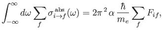
Thus, it follows that, provided state
is the ground state,
 |
(8.182) |
where
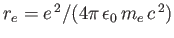 is the classical electron radius. Note that the integrated absorption cross-section is independent of Planck's constant. In fact, the previous result can also
be obtained from classical physics [67].
is the classical electron radius. Note that the integrated absorption cross-section is independent of Planck's constant. In fact, the previous result can also
be obtained from classical physics [67].
Next: Forbidden Transitions
Up: Time-Dependent Perturbation Theory
Previous: Spontaneous Emission of Radiation
Richard Fitzpatrick
2016-01-22