Next: Spontaneous Emission of Radiation
Up: Time-Dependent Perturbation Theory
Previous: Harmonic Perturbations
Absorption and Stimulated Emission of Radiation
Let us employ time-dependent perturbation theory
to investigate the interaction of an electron in a hydrogen-like atom with
classical (i.e., non-quantized) electromagnetic radiation.
The Hamiltonian of such an electron is
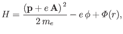 |
(8.122) |
where
 is the atomic potential energy, and
 and
and
 are the vector and scalar potentials associated with the
incident radiation. (See Section 3.6.)
The previous equation can be written
are the vector and scalar potentials associated with the
incident radiation. (See Section 3.6.)
The previous equation can be written
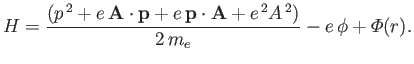 |
(8.123) |
Now,
 |
(8.124) |
provided that we adopt the Coulomb gauge,
 . (See Exercise 6.)
Hence,
. (See Exercise 6.)
Hence,
 |
(8.125) |
Suppose that the perturbation corresponds to a monochromatic plane-wave of angular frequency  , for which [49]
where
 and
and  are unit vectors that specify the wave's electric polarization direction (i.e., the direction of its
electric component)
and its direction of propagation, respectively. [The wavevector is
are unit vectors that specify the wave's electric polarization direction (i.e., the direction of its
electric component)
and its direction of propagation, respectively. [The wavevector is
 .] Here,
  is the velocity of light in vacuum.
Note that, according to standard electromagnetic theory,
is the velocity of light in vacuum.
Note that, according to standard electromagnetic theory,
 [49]. The Hamiltonian
becomes
[49]. The Hamiltonian
becomes
 |
(8.128) |
with
 |
(8.129) |
and
 |
(8.130) |
where the term involving  , which is second order in
  , has been neglected.
The perturbing Hamiltonian can be written
This has the same form as Equation (8.113), provided that
It is clear, by analogy with the analysis of Section 8.8, that the first
term on the right-hand side of Equation (8.134) describes a process by which the
atom absorbs energy
 from the electromagnetic field.
On the other hand, the second term describes a process by which the
atom emits energy
to the electromagnetic field.
We can interpret the former and latter processes as the absorption and stimulated emission, respectively, of a photon of energy
by the atom.
from the electromagnetic field.
On the other hand, the second term describes a process by which the
atom emits energy
to the electromagnetic field.
We can interpret the former and latter processes as the absorption and stimulated emission, respectively, of a photon of energy
by the atom.
It is convenient to define
![$\displaystyle {\bf d}_{if} = \frac{-{\rm i}}{m_e\,\omega_{if}}\left\langle i\le...
...\omega}{c}\right){\bf n}\cdot{\bf x}\right] {\bf p} \right\vert f\right\rangle,$](img2528.png) |
(8.133) |
which has the dimensions of length. Note that
  |
(8.134) |
It follows, from
Equations (8.122) and (8.123), that the rates of absorption and stimulated emission are
 |
(8.135) |
and
 |
(8.136) |
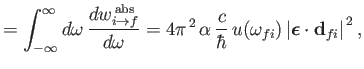
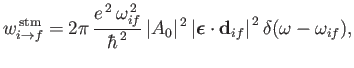
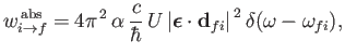
respectively. (See Exercise 19.) It can be seen that absorption involves the absorption by the atom of
a photon of angular frequency
 |
(8.137) |
and energy
 ,
causing a transition from an atomic state with an initial energy
,
causing a transition from an atomic state with an initial energy  to a state with a final energy
  .
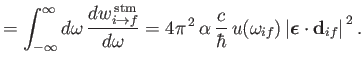
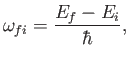
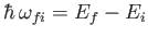
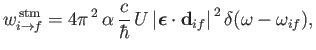
On the other hand, stimulated emission involves the emission by the atom of a photon of angular frequency
.
On the other hand, stimulated emission involves the emission by the atom of a photon of angular frequency
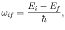 |
(8.138) |
and energy
 ,
causing a transition from an atomic state with an initial energy
to a state with a final energy
,
causing a transition from an atomic state with an initial energy
to a state with a final energy  .
In both cases,
and
specify the direction of propagation and electric polarization direction, respectively,
of the photon. For the case of stimulated emission,
and
also specify the direction of propagation and polarization direction, respectively, of the radiation that stimulates the atomic transition.
.
In both cases,
and
specify the direction of propagation and electric polarization direction, respectively,
of the photon. For the case of stimulated emission,
and
also specify the direction of propagation and polarization direction, respectively, of the radiation that stimulates the atomic transition.
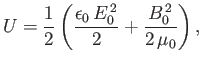
Now, the energy density of an electromagnetic radiation field
is [49]
 |
(8.139) |
where  and
and
 are the peak electric and magnetic field-strengths,
respectively. Hence,
are the peak electric and magnetic field-strengths,
respectively. Hence,
 |
(8.140) |
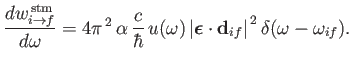
and expressions (8.138) and (8.139)
become
 |
(8.141) |
and
 |
(8.142) |
respectively,
where  is the fine structure constant.
Let us suppose that the incident radiation has a range of different angular frequencies, so
that
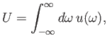 |
(8.143) |
where
 is the energy density of radiation whose angular frequency lies in the range
to
is the energy density of radiation whose angular frequency lies in the range
to
 . Equations (8.144) and (8.145) imply that
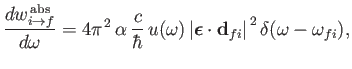 |
(8.144) |
and
 |
(8.145) |
Here,
 is the rate of absorption associated with
radiation whose angular frequency lies in the range
to
, et cetera.
Incidentally, we are assuming that the radiation is incoherent, so that intensities can be
added [64]. Of course,
is the rate of absorption associated with
radiation whose angular frequency lies in the range
to
, et cetera.
Incidentally, we are assuming that the radiation is incoherent, so that intensities can be
added [64]. Of course,
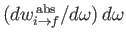
The rate at which the atom gains energy from the electromagnetic field as a consequence of absorption can be written
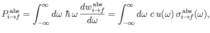 |
(8.148) |
where
 is the so-called absorption cross-section, and
 the
electromagnetic energy flux associated with radiation whose angular frequency lies in the range
to
[49]. It follows that
the
electromagnetic energy flux associated with radiation whose angular frequency lies in the range
to
[49]. It follows that
 |
(8.149) |
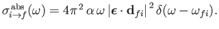
Similarly, the stimulated emission cross-section takes the form
 |
(8.150) |
Finally, comparing Equations (8.149) and (8.150) with the previous two equations, we deduce that
Here, we have written
 , where
 is the number density of
photons whose angular frequencies lie in the range
to
.
is the number density of
photons whose angular frequencies lie in the range
to
.
Next: Spontaneous Emission of Radiation
Up: Time-Dependent Perturbation Theory
Previous: Harmonic Perturbations
Richard Fitzpatrick
2016-01-22
![$\displaystyle V = \frac{e \,A_0}{m_e}\, \exp\left[-{\rm i}\left(\frac{\omega}{c}\right) {\bf n}\cdot{\bf x}\right]$](img2527.png)
![$\displaystyle H_1 = \frac{e \,A_0}{m_e} \left(\exp\left[\,{\rm i}\left(\frac{\o...
...frac{\omega}{c}\right) {\bf n}\cdot{\bf x} + {\rm i}\, \omega\, t\right]\right)$](img2525.png)