Next: Absorption and Stimulated Emission
Up: Time-Dependent Perturbation Theory
Previous: Energy-Shifts and Decay-Widths
Harmonic Perturbations
Consider a perturbation to the Hamiltonian that oscillates sinusoidally in time.
This is usually termed a harmonic perturbation. Thus,
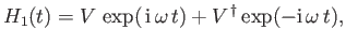 |
(8.110) |
where  is, in general, a function of the position, momentum, and
spin operators.
is, in general, a function of the position, momentum, and
spin operators.
Let us initiate the system in the eigenstate  of the unperturbed
Hamiltonian,
of the unperturbed
Hamiltonian,  , and then switch on the harmonic perturbation at
  .
It follows from Equation (8.59) that
.
It follows from Equation (8.59) that
where
Equation (8.114) is analogous to Equation (8.66), provided that
 |
(8.114) |
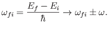
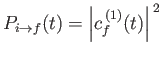
Thus, it follows from the analysis of Section 8.6 that
the transition probability
 is only appreciable in the limit
 if
if
Clearly, criterion (8.118) corresponds to the first term on the right-hand side
of Equation (8.114), whereas criterion (8.119) corresponds to the second. The former
term describes a process by which the system gives up energy
 to the perturbing field, while making a transition
to a final state whose energy is less than that of the initial
state by
. This process is known as stimulated emission.
The latter term describes a process by which the system gains
energy
from the perturbing field, while making a transition
to a final state whose energy exceeds that of the initial
state by
. This process is known as absorption. In
both cases, the total energy (i.e., that of the system plus
the perturbing field) is conserved.
to the perturbing field, while making a transition
to a final state whose energy is less than that of the initial
state by
. This process is known as stimulated emission.
The latter term describes a process by which the system gains
energy
from the perturbing field, while making a transition
to a final state whose energy exceeds that of the initial
state by
. This process is known as absorption. In
both cases, the total energy (i.e., that of the system plus
the perturbing field) is conserved.
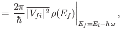
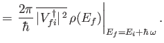
By analogy with Equation (8.79),
Equation (8.120) specifies the transition rate for stimulated emission, whereas
Equation (8.121) gives the transition rate for absorption.
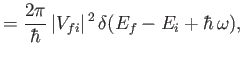
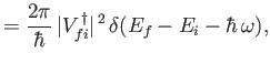
These transition rates are more usually written [see Equation (8.80)]
where it is understood that the previous expressions must be integrated with
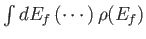 to obtain the actual transition rates.
It is clear from Equations (8.115) and (8.116) that
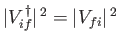 .
It follows from Equations (8.120) and (8.121) that
.
It follows from Equations (8.120) and (8.121) that
![$\displaystyle \frac{w_{i\rightarrow [f]}^{\,\rm stm}}{\rho(E_f)} = \frac{w_{f\rightarrow [i]}^{\,\rm abs}}{\rho(E_i)}.$](img2505.png) |
(8.121) |
In other words, the rate of stimulated emission, divided by the density
of final states for stimulated emission, is equal to the rate of absorption,
divided
by the density of final states for absorption. This result, which
expresses a fundamental symmetry between absorption and stimulated
emission, is known as detailed balance, and plays an important role in
quantum statistical mechanics.
Next: Absorption and Stimulated Emission
Up: Time-Dependent Perturbation Theory
Previous: Energy-Shifts and Decay-Widths
Richard Fitzpatrick
2016-01-22
![$\displaystyle = \left(\frac{-{\rm i}}{\hbar}\right) \int_0^t dt'\left[V_{fi} \,...
...\dagger}\, \exp(-{\rm i}\,\omega\, t')\right]\exp(\,{\rm i}\, \omega_{fi}\, t')$](img2483.png)
![$\displaystyle = \frac{1}{\hbar} \left(\frac{1-\exp[\,{\rm i}\,(\omega_{fi} + \o...
...,(\omega_{fi}-\omega )\,t]} {\omega_{fi} - \omega} \,V_{fi}^{\,\dagger}\right),$](img2484.png)