


Next: Energy-Shifts and Decay-Widths
Up: Time-Dependent Perturbation Theory
Previous: Dyson Series
Sudden Perturbations
Consider, for example, a constant perturbation that is suddenly switched on at time
 : that is,
![$\displaystyle H_1(t)=\left\{ \begin{array}{lll} 0 &\mbox{\hspace{0.5cm}}&\mbox{for $t<0$} \\ [0.5ex] H_1&&\mbox{for $t\geq 0$}\end{array}\right.,$](img2366.png) |
(8.61) |
where  is independent of time, but is generally a function of
the position,
momentum, and spin operators. Suppose that the system is definitely
in state
is independent of time, but is generally a function of
the position,
momentum, and spin operators. Suppose that the system is definitely
in state  at time
. According to Equations (8.58) and (8.59) (with
at time
. According to Equations (8.58) and (8.59) (with
 ),
),
giving
![$\displaystyle P_{i\rightarrow f}(t) \simeq \left\vert c_f^{\,(1)}(t)\right\vert...
...vert E_f - E_i\vert^{\,2}}\, \sin^2\left[ \frac{(E_f-E_i)\,t}{2\,\hbar}\right],$](img2368.png) |
(8.64) |
for  .
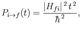
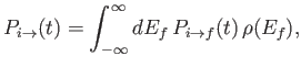
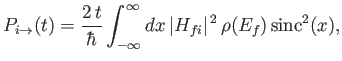
The transition probability between states
and
.
The transition probability between states
and  can be written
![$\displaystyle P_{i\rightarrow f}(t) = \frac{\vert H_{fi}\vert^{\,2} \,t^{\,2}}{\hbar^{\,2}} \,{\rm sinc}^2\left[ \frac{(E_f-E_i)\,t}{2\,\hbar}\right],$](img2369.png) |
(8.65) |
where
 |
(8.66) |
The sinc function is highly oscillatory, and decays like  at large
  . In fact, it is a good approximation to say that
 is small compared to unity except when
 . It follows that the
transition probability,
. It follows that the
transition probability,
 , is negligibly small unless
 |
(8.67) |
Note that, in the limit
 , only those transitions
that conserve energy (i.e.,
, only those transitions
that conserve energy (i.e.,  ) have an appreciable
probability of occurrence. At finite
) have an appreciable
probability of occurrence. At finite  , is is possible to
have transitions that do not exactly conserve energy, provided that
, is is possible to
have transitions that do not exactly conserve energy, provided that
 |
(8.68) |
where
 is the change in energy of the system associated
with the transition, and
is the change in energy of the system associated
with the transition, and
 is the time elapsed since the
perturbation was switched on. This result is a manifestation
of the well-known uncertainty relation for energy and time [53]. Incidentally, the energy-time
uncertainty relation is fundamentally different from the position-momentum
uncertainty relation because (in non-relativistic quantum mechanics)
position and momentum are operators, whereas time is merely a parameter.
is the time elapsed since the
perturbation was switched on. This result is a manifestation
of the well-known uncertainty relation for energy and time [53]. Incidentally, the energy-time
uncertainty relation is fundamentally different from the position-momentum
uncertainty relation because (in non-relativistic quantum mechanics)
position and momentum are operators, whereas time is merely a parameter.
The probability of a transition that conserves energy (i.e.,
)
is
 |
(8.69) |
where use has been made of
 . Note that this probability
grows quadratically in time. This result is somewhat surprising, because
it implies that the probability of a transition occurring in a fixed
time interval,
to
. Note that this probability
grows quadratically in time. This result is somewhat surprising, because
it implies that the probability of a transition occurring in a fixed
time interval,
to  , grows linearly with
, despite the fact that
is constant for
, grows linearly with
, despite the fact that
is constant for  . In practice, there is usually a group of
final states, all possessing nearly the same energy as the energy of the
initial state,
. It is helpful to define the density of
states,
. In practice, there is usually a group of
final states, all possessing nearly the same energy as the energy of the
initial state,
. It is helpful to define the density of
states,  , where the number of final states lying in the
energy range
, where the number of final states lying in the
energy range  to
to  is given by
 . Thus, the
probability of a transition from the initial state
to one of
the continuum of possible final states is
. Thus, the
probability of a transition from the initial state
to one of
the continuum of possible final states is
 |
(8.70) |
giving
 |
(8.71) |
where
 |
(8.72) |
and use has been made of Equation (8.68). We know that, in the limit
, the function
is only non-zero in an infinitesimally
narrow range of final energies centered on
. It follows that, in this limit,
we can take
 and
and
 out of the integral in the previous
formula to obtain
out of the integral in the previous
formula to obtain
![$\displaystyle P_{i\rightarrow[f]} (t) = \left.\frac{2\pi}{\hbar}\, \overline{\vert H_{fi}\vert^{\,2}} \,\rho(E_f)\,t\, \right\vert _{E_f\simeq E_i},$](img2394.png) |
(8.73) |
where
![$ P_{i\rightarrow [f]}$](img2395.png) denotes the transition probability between
the initial state,
,
and all final states,
, that have approximately the same energy
as the initial state.
Here,
denotes the transition probability between
the initial state,
,
and all final states,
, that have approximately the same energy
as the initial state.
Here,
 is the average of
over
all final states with approximately the same energy as the initial state.
In deriving the previous formula, we have made use of the result [59]
is the average of
over
all final states with approximately the same energy as the initial state.
In deriving the previous formula, we have made use of the result [59]
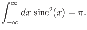 |
(8.74) |
Note that the transition probability,
,
is now proportional to
, instead
of  .
.
It is convenient to define the transition rate, which is simply
the transition probability per unit time. Thus,
![$\displaystyle w_{i\rightarrow [f]} = \frac{d P_{i\rightarrow [f]}}{dt},$](img2399.png) |
(8.75) |
which implies that
![$\displaystyle w_{i\rightarrow [f]} = \left.\frac{2\pi}{\hbar}\, \overline{\vert H_{fi}\vert^{\,2}} \,\rho(E_f) \right\vert _{E_f\simeq E_i}.$](img2400.png) |
(8.76) |
This appealingly simple result is known as Fermi's golden rule [29,44].
Note that the transition rate is constant in time (for
):
that is, the probability of a transition occurring in the time interval
to
is independent of
for fixed  .
Fermi's golden rule is more usually written
.
Fermi's golden rule is more usually written
 |
(8.77) |
where it is understood that this formula must be integrated
with
 in order to obtain the actual transition rate.
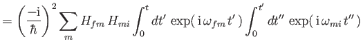
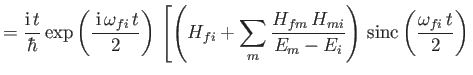
Let us now calculate the second-order term in the Dyson series, using the
constant perturbation (8.64). From Equation (8.60), we find that (with
)
Thus,
where use has been made of Equation (8.66). It follows, by analogy with the
previous analysis, that
![$\displaystyle w_{i\rightarrow [f]} =\left. \frac{2\pi}{\hbar}\, \overline{ \lef...
...\,H_{mi}}{E_m - E_i}\right\vert^{\,2}} \rho(E_f) \right\vert _{E_f \simeq E_i},$](img2410.png) |
(8.80) |
where the transition rate is calculated for all final states,
, with
approximately the same energy as the initial state,
, and for
intermediate states,  whose energies differ from that of
the initial state. The fact that
whose energies differ from that of
the initial state. The fact that
 causes the final term on the
right-hand side of Equation (8.82) to average to zero during the evaluation of the transition probability. (See Exercise 4.)
causes the final term on the
right-hand side of Equation (8.82) to average to zero during the evaluation of the transition probability. (See Exercise 4.)
According to Equation (8.83), a second-order transition takes place in
two steps. First, the system makes a non-energy-conserving transition to
some intermediate state
. Subsequently, the system makes another
non-energy-conserving transition to the final state
. The net
transition from state
to state
conserves energy. The
non-energy-conserving transitions are generally termed virtual
transitions, whereas the energy conserving first-order transition
is termed a real transition. The previous formula clearly breaks down
if
 when
when
 . This problem can be avoided by
gradually turning on the perturbation: that is,
. This problem can be avoided by
gradually turning on the perturbation: that is,
 (where
  is very small). The net result is to change the energy
denominator in Equation (8.83) from
is very small). The net result is to change the energy
denominator in Equation (8.83) from  to
to
 .
.
Next: Energy-Shifts and Decay-Widths
Up: Time-Dependent Perturbation Theory
Previous: Dyson Series
Richard Fitzpatrick
2016-01-22
![$\displaystyle = -\frac{{\rm i}}{\hbar}\, H_{fi} \int_0^t dt'\,\exp[\,{\rm i}\, ...
...{fi}\,(t'-t)]= \frac{H_{fi}}{E_f - E_i}\, [1- \exp(\,{\rm i}\,\omega_{fi}\,t)],$](img2367.png)
![$\displaystyle =\frac{\rm i}{\hbar} \sum_m \frac{H_{fm} \,H_{mi}}{E_m - E_i} \in...
...[\exp(\,{\rm i}\,\omega_{fi}\,t'\,) - \exp(\,{\rm i}\,\omega_{fm}\,t')\,\right]$](img2405.png)
![$\displaystyle = \frac{{\rm i}\,t}{\hbar} \sum_m \frac{H_{fm} \,H_{mi}}{E_m - E_...
...a_{fm} \,t}{2}\right) \,{\rm sinc}\left(\frac{\omega_{fm}\,t}{2}\right)\right].$](img2406.png)
![$\displaystyle \left. - \sum_m\frac{H_{fm}\,H_{mi}}{E_m - E_i} \exp\left(\frac{\...
...ega_{im}\,t}{2}\right)\,{\rm sinc}\left(\frac{\omega_{fm}\,t}{2}\right)\right],$](img2409.png)