Quadratic Stark Effect

The Stark effect is a phenomenon by which the energy eigenstates of an atomic or molecular system are modified in the presence of a static, external, electric field. This phenomenon was first observed experimentally (in hydrogen) by J. Stark in 1913 [105]. Let us employ perturbation theory to investigate the Stark effect.

Suppose that a hydrogen-like atom [i.e., either a hydrogen atom, or an alkali metal atom (which possesses one valance electron orbiting outside a closed, spherically symmetric, shell)] is subjected to a uniform electric field, ${\bf E}$ , pointing in the positive $z$ -direction. The Hamiltonian of the system can be split into two parts. The unperturbed Hamiltonian,

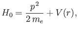$$H_0 = \frac{p^{\,2}}{2\,m_e} + V(r),$$ (7.38)

and the perturbing Hamiltonian,

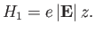$$H_1= e\, \vert{\bf E}\vert\, z.$$ (7.39)

It is assumed that the unperturbed energy eigenvalues and eigenstates are completely known. The electron spin is irrelevant in this problem (because the spin operators all commute with $H_1$ ), so we can ignore the spin degrees of freedom of the system. This implies that the system possesses no degenerate energy eigenvalues. Actually, this is not true for the $n\neq 1$ energy levels of the hydrogen atom, because of the special properties of a pure Coulomb potential. (See Section 4.6.) It is necessary to deal with this case separately, because the perturbation theory presented in Section 7.3 breaks down for degenerate unperturbed energy levels. (See Section 7.5.)

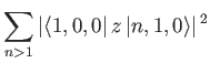
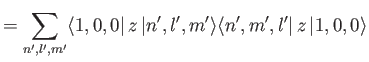
An energy eigenket of the unperturbed Hamiltonian is characterized by three quantum numbers--the principal quantum number $n$ , and the azimuthal and magnetic quantum numbers, $l$ and $m$ , respectively. (See Section 4.6.) Let us denote such a ket $\vert n,l,m\rangle$ , and let its energy be $E_{nlm}$ . According to Equation (7.32), the change in this energy induced by a small external electric field (i.e., small compared to the typical electric field internal to the atom) is given by

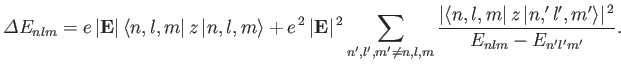$${\mit\Delta} E_{nlm}=e\,\vert{\bf E}\vert\, \langle n,l,m \vert\,... ...\langle n,l,m\vert\,z\,\vert n,'l',m'\rangle\vert^{\,2}}{ E_{nlm}-E_{n'l'm'} }.$$ (7.40)

Now, because

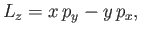$$L_z = x\,p_y - y\, p_x,$$ (7.41)

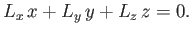
it follows that

$$[L_z, z] = 0.$$ (7.42)

(See Chapter 4.) Thus,

$$\langle n,l, m\vert\, [L_z, z]\, \vert n',l',m'\rangle = 0,$$ (7.43)

giving

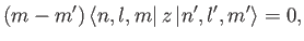$$(m - m')\, \langle n,l, m\vert\,z\,\vert n',l',m'\rangle = 0,$$ (7.44)

because $\vert n,l,m\rangle$ is, by definition, an eigenstate of $L_z$ corresponding to the eigenvalue $m\,\hbar$ . It is clear, from the previous equation, that the matrix element $\langle n,l, m\vert\,z\,\vert n',l',m'\rangle$ is zero unless $m'=m$ . This is termed the selection rule for the magnetic quantum number, $m$ .

Let us now determine the selection rule for the azimuthal quantum number, $l$ . We have

$$[L^2, z] = [L_x^{\,2}, z] + [L_y^{\,2}, z] = L_x\,[L_x, z] + [L_x, z] \,L_x + L_y\,[L_y, z] + [L_y, z]\, L_y$$

$$= {\rm i}\,\hbar\left( -L_x\, y - y\, L_x + L_y \,x + x \,L_y\right)= 2 \,{\rm i} \, \hbar \,( L_y \,x - L_x \,y + {\rm i}\,\hbar\,z)$$

$$= 2 \,{\rm i}\, \hbar \,( L_y\, x - y \,L_x ) = 2\, {\rm i}\, \hbar\, ( x\, L_y - L_x \,y),$$ (7.45)

where use has been made of Equations (4.1)-(4.6). Similarly,

$$[L^2, y] = 2\,{\rm i}\, \hbar \,( L_x\, z - x\, L_z ),$$ (7.46)

$$[L^2, x] = 2\,{\rm i}\, \hbar\, ( y \,L_z - L_y \,z).$$ (7.47)

Thus,

$$[L^2, [L^2, z]] = 2 \,{\rm i} \, \hbar \left( L^2, L_y \,x - L_x\, y + {\rm i}\,\hbar\,z \right)$$

$$= 2\,{\rm i}\,\hbar \left( L_y\, [L^2, x] - L_x\, [ L^2, y] + {\rm i}\,\hbar\, [L^2, z]\right)$$

$$= - 4\, \hbar^{\,2} \,L_y\,(y\, L_z - L_y \,z) + 4\,\hbar^2 \,L_x\,(L_x\, z - x\, L_z)$$

$$\phantom{=}- 2\, \hbar^2\,(L^2 \,z - z\, L^2).$$ (7.48)

This reduces to

$$[L^2, [L^2, z]] = - \hbar^{\,2} \left[4\,(L_x\, x + L_y \,y + L_z \,z)\, L_z - 4\, (L_x^{\,2} + L_y^{\,2} + L_z^{\,2})\, z \right.$$

$$\phantom{L}\left.+ 2 \,(L^2\, z - z\, L^2)\right].$$ (7.49)

However, it is clear from Equations (4.1)-(4.3) that

$$L_x \,x + L_y \,y + L_z \,z = 0.$$ (7.50)

Hence, we obtain

$$[L^2, [L^2, z]] = 2 \,\hbar^2\, (L^2\, z + z \,L^2),$$ (7.51)

which can be expanded to give

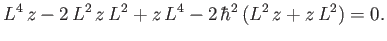$$L^4 \,z - 2\, L^2 \,z\, L^2 + z\, L^4 - 2\, \hbar^2\, (L^2 \,z +z \,L^2) = 0.$$ (7.52)

Equation (7.52) implies that

$$\langle n,l,m\vert\, L^4\, z - 2\, L^2\, z \,L^2 + z\, L^4 - 2 \,\hbar^{\,2} \,(L^2\, z +z\, L^2)\, \vert n',l',m' \rangle = 0.$$ (7.53)

Because $\vert n,l,m\rangle$ is, by definition, an eigenstate of $L^2$ corresponding to the eigenvalue $l\,(l+1)\,\hbar^{\,2}$ , the previous expression yields

$$\begin{multline} \left[l^{\,2}\, (l+1)^2 - 2\, l\,(l+1)\,l'\,(l'+1) + l'^{\,2}\,... ...,(l'+1)\right] \langle n,l,m\vert\,z\,\vert n',l',m' \rangle = 0, \end{multline}$$

which reduces to

$$(l+l'+2)\,(l+l')\,(l-l'+1)\,(l-l'-1)\,\langle n,l,m\vert\,z\,\vert n',l',m' \rangle = 0.$$ (7.54)

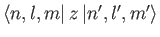
According to the previous formula, the matrix element $\langle n,l, m\vert\,z\,\vert n',l',m'\rangle$ vanishes unless $l=l'=0$ or $l' = l\pm 1$ . This matrix element can be written

$$\langle n,l,m\vert\,z\,\vert n',l',m' \rangle = \int\!\!\int\!\!\... ...nlm}(r',\theta',\varphi')\, r'\cos\theta'\, \psi_{n'm'l'}(r',\theta',\varphi'),$$ (7.55)

where $\psi_{nlm}({\bf x}') = \langle {\bf x}'\vert n,l,m\rangle$ . Recall, however, that the wavefunction of an $l=0$ state is spherically symmetric: that is, $\psi_{n00}({\bf x}') = \psi_{n00}(r')$ . (See Section 4.3.) It follows from Equation (7.56) that the matrix element vanishes, by symmetry, when $l=l'=0$ . In conclusion, the matrix element $\langle n,l, m\vert\,z\,\vert n',l',m'\rangle$ is zero unless $l' = l\pm 1$ . This is the selection rule for the quantum number $l$ .

Application of the previously derived selection rules for $m$ and $l$ to Equation (7.40) yields

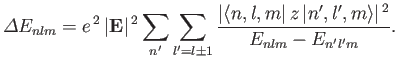$${\mit\Delta} E_{nlm} = e^{\,2} \,\vert{\bf E}\vert^{\,2} \sum_{n'... ...t\langle n,l,m\vert\,z\,\vert n',l',m\rangle\vert^{\,2}}{E_{nlm} - E_{n'l' m}}.$$ (7.56)

Note that all of the terms appearing in Equation (7.40) that vary linearly with the electric field-strength vanish, by symmetry, according to the selection rules. Only those terms that vary quadratically with the field-strength survive. Hence, the energy-shift specified in the previous formula is known as the quadratic Stark effect.

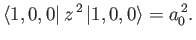
The electrical polarizability, $\alpha_p$ , of an atom is defined in terms of the electric-field-induced energy-shift of a given atomic state as follows [67]:

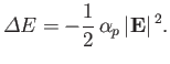$${\mit\Delta} E = - \frac{1}{2} \,\alpha_p \,\vert{\bf E}\vert^{\,2}.$$ (7.57)

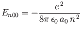
Consider the ground state of a hydrogen atom. (Recall, that we cannot address the $n>1$ excited states because they are degenerate, and our theory cannot deal with this at present). The polarizability of the ground state is given by

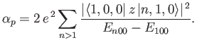$$\alpha_p = 2 \,e^{\,2} \sum_{n>1} \frac{\vert\langle 1,0,0\vert\,z\,\vert n,1,0\rangle\vert^{\,2}}{E_{n00}-E_{100}}.$$ (7.58)

Here, we have made use of the fact that $E_{n10} = E_{n00}$ for a hydrogen atom. (See Section 4.6.)

The sum in the previous expression can be evaluated approximately by noting that

$$E_{n00} = - \frac{e^{\,2}}{8\pi\,\epsilon_0\, a_0\,n^{\,2}}$$ (7.59)

for a hydrogen atom, where $a_0$ is the Bohr radius. [See Equation (4.132).] We can write

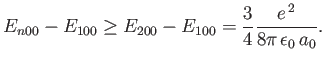$$E_{n00}-E_{100} \geq E_{200} - E_{100} = \frac{3}{4} \frac{e^{\,2}}{8\pi\,\epsilon_0\, a_0}.$$ (7.60)

Thus,

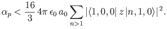$$\alpha_p < \frac{16}{3}\, 4\pi \,\epsilon_0\, a_0 \sum_{n>1} \vert\langle 1,0,0\vert\,z\,\vert n,1,0\rangle\vert^{\,2}.$$ (7.61)

However,

$$\sum_{n>1} \vert\langle 1,0,0\vert\,z\,\vert n,1,0\rangle\vert^{\,2} = \sum_{n',l',m'} \langle 1,0,0\vert\,z\,\vert n',l',m'\rangle\langle n',m',l'\vert\,z\,\vert 1,0,0\rangle$$

$$= \langle 1,0,0\vert\,z^{\,2}\,\vert 1,0,0\rangle,$$ (7.62)

where we have made use of the fact that the wavefunctions of a hydrogen atom form a complete set. It is easily demonstrated from the actual form of the ground-state wavefunction that

$$\langle 1,0,0\vert\,z^{\,2}\,\vert 1,0,0\rangle = a_0^{\,2}.$$ (7.63)

(See Exercise 13.) Thus, we conclude that

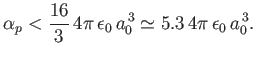$$\alpha_p < \frac{16}{3} \,4\pi\, \epsilon_0\, a_0^{\,3} \simeq 5.3\,4\pi\, \epsilon_0 \,a_0^{\,3}.$$ (7.64)

The exact result is

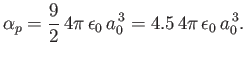$$\alpha_p = \frac{9}{2}\, 4\pi\, \epsilon_0\, a_0^{\,3} = 4.5\,4\pi \,\epsilon_0 \,a_0^{\,3}.$$ (7.65)

It is possible to obtain this result, without recourse to perturbation theory, by solving Schrödinger's equation in parabolic coordinates [115,41].