Next: Flux Quantization and the
Up: Quantum Dynamics
Previous: Charged Particle Motion in
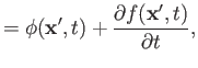
In the Schrödinger picture, the Hamiltonian (3.71) leads to the following time-dependent
wave equation:
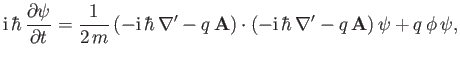 |
(3.89) |
where
 ,
,
 , and
, and
 .
Now, the Heisenberg equation of motion (3.88) only involves the electric and magnetic fields, and is independent of the
vector and scalar potentials. On the other hand, the previous wave equation involves the potentials, but not the fields.
As is well known, the vector and scalar potentials are not well defined, in that there are many different
potentials that generate the same electric and magnetic fields. To be more exact, a transformation of the
form
.
Now, the Heisenberg equation of motion (3.88) only involves the electric and magnetic fields, and is independent of the
vector and scalar potentials. On the other hand, the previous wave equation involves the potentials, but not the fields.
As is well known, the vector and scalar potentials are not well defined, in that there are many different
potentials that generate the same electric and magnetic fields. To be more exact, a transformation of the
form
 and
and
 , where
and
 is an arbitrary function, leaves the
  and
and  fields unaffected.
Such a transformation is known as a gauge transformation.
It is evident that a gauge transformation would leave the Heisenberg equation of motion (3.88) unchanged,
but would modify the time-dependent wave equation (3.89). However, these two
equations are supposed to give results that are consistent with one another. Let us investigate how this is possible.
fields unaffected.
Such a transformation is known as a gauge transformation.
It is evident that a gauge transformation would leave the Heisenberg equation of motion (3.88) unchanged,
but would modify the time-dependent wave equation (3.89). However, these two
equations are supposed to give results that are consistent with one another. Let us investigate how this is possible.
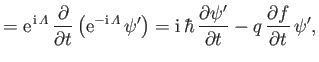
The previous three equations can be combined to give
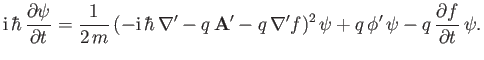 |
(3.92) |
Let
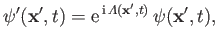 |
(3.93) |
where
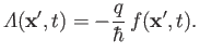 |
(3.94) |
It follows that
Hence, Equation (3.92) becomes
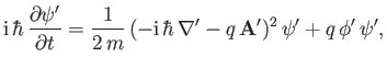 |
(3.98) |
which is analogous in form to Equation (3.89). Thus, we deduce that if
and
then
 . In other words, a gauge transformation introduces a position- and
time-dependent phase-shift,
. In other words, a gauge transformation introduces a position- and
time-dependent phase-shift,
 , into the wavefunction.
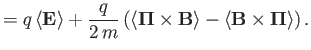
Now, Equation (3.88) is equivalent to Equations (3.76) and (3.87).
If we take the expectation values of the latter two equations then we obtain
However, the quantities
 ,
,


 ,
,
 ,
,
 , and
, and
 are all
invariant under the gauge transformation
,
, and
. This follows because
are all
invariant under the gauge transformation
,
, and
. This follows because
et cetera. Thus, Equations (3.88) and (3.89) do indeed give consistent results under
gauge transformation.
Next: Flux Quantization and the
Up: Quantum Dynamics
Previous: Charged Particle Motion in
Richard Fitzpatrick
2016-01-22


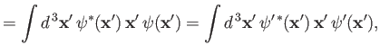
![$\displaystyle = \int d^{\,3}{\bf x}'\,\psi^\ast({\bf x}')\left[-{\rm i}\,\hbar\,\nabla' -q\,{\bf A}({\bf x}')\right]\psi({\bf x}')$](img800.png)
![$\displaystyle = \int d^{\,3}{\bf x}'\,\psi'^{\,\ast}({\bf x}') \left[-{\rm i}\,\hbar\,\nabla' -q\, {\bf A}'({\bf x}')\right]\psi'({\bf x}'),$](img801.png)