Next: Classical Closure Scheme Up: Plasma Fluid Theory Previous: Fundamental Quantities Contents
 (because collisions conserve momentum) [18].
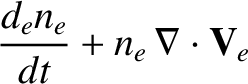
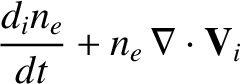
In their present forms, the electron and ion fluid equations
relate interesting fluid quantities, such as the electron number density,
(because collisions conserve momentum) [18].
In their present forms, the electron and ion fluid equations
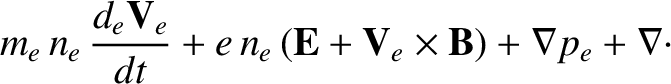
relate interesting fluid quantities, such as the electron number density,  , the mean
flow velocities,
, the mean
flow velocities,  and
and  , and the scalar pressures,
  and
and  , to unknown quantities,
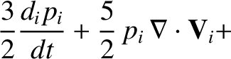
such as the viscosity tensors,
, to unknown quantities,
such as the viscosity tensors,

 and
and
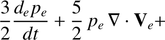
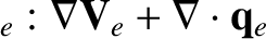
 , the heat fluxes,
  and
and  , and the
moments of the collision operator,
, and the
moments of the collision operator,  ,
,  , and
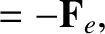
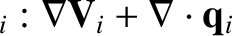
, and  . In order to complete
our set of equations, we need to employ some additional information to express the
latter quantities in terms of the former; this process is known as closure.
. In order to complete
our set of equations, we need to employ some additional information to express the
latter quantities in terms of the former; this process is known as closure.
There are two basic types of fluid closure schemes. In truncation schemes, high-order velocity-space moments of the distribution function are assumed to vanish, or are prescribed in terms of low-order moments [24,36]. Truncation schemes are relatively straightforward to implement, but the error associated with the closure cannot easily be determined. Asymptotic schemes, on the other hand, depend on a rigorous expansion of the kinetic equation in terms of some dimensionless parameter that is small compared to unity [10]. Asymptotic closure schemes have the advantage of providing some estimate of the error involved in the closure. However, the asymptotic approach to closure is mathematically demanding, because it involves working closely with the kinetic equation. In this book, we shall rely on a mixture of truncation and asymptotic closure schemes.