Next: MHD Equations Up: Plasma Fluid Theory Previous: Normalization of Braginskii Equations Contents
 ,
to derive the cold-plasma equations:
and
Let us now use the smallness of the mass ratio
,
to derive the cold-plasma equations:
and
Let us now use the smallness of the mass ratio  to further
simplify these equations. In particular, we would like to write the
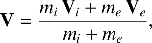
electron and ion fluid velocities in terms of the center-of-mass
velocity,
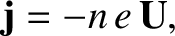
and the plasma current
where
to further
simplify these equations. In particular, we would like to write the
electron and ion fluid velocities in terms of the center-of-mass
velocity,
and the plasma current
where
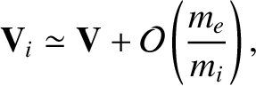
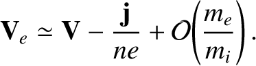
 . According to the ordering
scheme adopted in the previous section,
. According to the ordering
scheme adopted in the previous section,
 in the cold-plasma
limit. We shall continue to regard the mean-free-path parameter
in the cold-plasma
limit. We shall continue to regard the mean-free-path parameter  as
as
 .
.
It follows from Equations (4.179) and (4.180) that
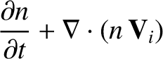
andEquations (4.175), (4.177), (4.181), and (4.182) yield the continuity equation:
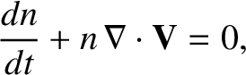 |
(4.183) |
 . Here, use has
been made of the fact that
. Here, use has
been made of the fact that
 in a quasi-neutral
plasma.
in a quasi-neutral
plasma.
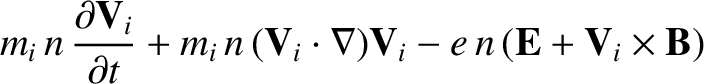
Equations (4.176) and (4.178) can be summed to give the equation of motion:
 |
(4.184) |
Finally, Equations (4.176), (4.181), and (4.182) can be combined to give a modified Ohm's law:
 |
 |
(4.185) |

![$\displaystyle = [\zeta]\,{\bf F}_U,$](img1438.png)
![$\displaystyle =- [\zeta]\,{\bf F}_U.$](img1440.png)