Next: Plasma Dispersion Function Up: Waves in Warm Plasmas Previous: Landau Damping Contents
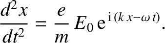
![$E_0\,\exp[\,{\rm i}\,
(k\,x-\omega\,t)]$](img2303.png) is determined by
is determined by
 |
(7.33) |
 at position
  then we may substitute
 for
for  in the electric field term. This is actually the position of
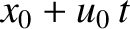
the particle on its unperturbed trajectory, starting at
in the electric field term. This is actually the position of
the particle on its unperturbed trajectory, starting at  at
at  .
Thus, we obtain
.
Thus, we obtain
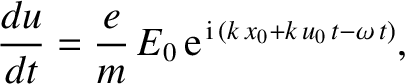 |
(7.34) |
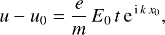
![$\displaystyle u-u_0 = \frac{e}{m}\,E_0\left[\frac{{\rm e}^{\,{\rm i}\,(k\,x_0+k...
...,t-\omega\,t)}
- {\rm e}^{\,{\rm i}\,k\,x_0}}{{\rm i}\,(k\,u_0-\omega)}\right].$](img2308.png) |
(7.35) |
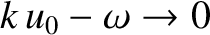 , the previous expression reduces to
 |
(7.36) |
close to  —that is, with velocity
components along the -axis close to the phase-velocity of the wave—have
velocity perturbations that grow in time. These so-called resonant particles
gain energy from, or lose energy to, the wave, and are responsible for the
damping. This explains why the damping rate, given by Equation (7.31), depends on the
slope of the distribution function calculated at
—that is, with velocity
components along the -axis close to the phase-velocity of the wave—have
velocity perturbations that grow in time. These so-called resonant particles
gain energy from, or lose energy to, the wave, and are responsible for the
damping. This explains why the damping rate, given by Equation (7.31), depends on the
slope of the distribution function calculated at
 . The remainder of the
particles are non-resonant, and have an oscillatory response to the
wave field.
. The remainder of the
particles are non-resonant, and have an oscillatory response to the
wave field.
To understand why energy should be transferred from the electric field to the resonant particles requires more detailed consideration (Cairns 1985). Whether the speed of a resonant particle increases or decreases depends on the phase of the wave at its initial position, and it is not the case that all particles moving slightly faster than the wave lose energy, while all particles moving slightly slower than the wave gain energy. Furthermore, the density perturbation oscillates out of phase with the wave electric field, so there is no initial wave-generated excess of particles gaining or losing energy. However, if we consider those particles that start off with velocities slightly above the phase-velocity of the wave then if they gain energy they move away from the resonant velocity whereas if they lose energy they approach the resonant velocity. The result is that the particles which lose energy interact more effectively with the wave, and, on average, there is a transfer of energy from these particles to the electric field. Exactly the opposite is true for particles with initial velocities lying just below the phase-velocity of the wave. In the case of a Maxwellian distribution, there are more particles in the latter class than in the former, so there is a net transfer of energy from the electric field to the particles: that is, the electric field is damped. In the limit that the wave amplitude tends to zero, it is clear that the damping rate is determined by velocity gradient of the distribution function at the wave speed.
The previous argument fails if
the magnitude of the initial electric field becomes too large, because nonlinear effects become important (Cairns 1985). The basic
requirement for the validity of the linear result is that a resonant
particle should maintain its position relative to the phase of the
electric field over a sufficiently long time period for the damping to
take place. To determine the condition that this be the case, let us consider the
problem in the frame of reference in which the wave is at rest, and the
potential
 seen by an electron is as sketched in Figure 7.5.
If the electron starts at rest (i.e., in resonance with the wave) at
then it begins to move towards the potential minimum, as shown. The time for
the electron to shift its position relative to the wave may be estimated
as the period with which it bounces back and forth in the potential well.
Near the bottom of the well, the equation of motion of the electron is written
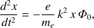 |
(7.37) |
 is the wavenumber, and
 is the amplitude of the potential. Thus, the bounce time is
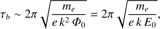 |
(7.38) |
 is the amplitude of the electric field. We may expect the wave
to damp according to linear theory if the bounce time,
is the amplitude of the electric field. We may expect the wave
to damp according to linear theory if the bounce time,  , is much greater than the damping time. Because the former time varies
inversely with the square root of the electric field amplitude, whereas the
latter is amplitude independent, this criterion gives us an estimate of
the maximum allowable initial electric field amplitude that is consistent with linear
damping (Cairns 1985).
, is much greater than the damping time. Because the former time varies
inversely with the square root of the electric field amplitude, whereas the
latter is amplitude independent, this criterion gives us an estimate of
the maximum allowable initial electric field amplitude that is consistent with linear
damping (Cairns 1985).
If the initial amplitude is large enough for the resonant electrons to
bounce back and forth in the potential well a number of times before the
wave is damped then it can be demonstrated that the result to be expected is
a non-monotonic decrease in the amplitude of the electric field, as shown
in Figure 7.6 (O'Neil 1965; Armstrong 1967). The period of the amplitude oscillations is similar to the bounce
time, .
![\includegraphics[height=2.5in]{Chapter07/fig7_5.eps}](img2313.png)
![\includegraphics[height=2.5in]{Chapter07/fig7_6.eps}](img2317.png)