Next: Perpendicular Wave Propagation Up: Waves in Cold Plasmas Previous: Low-Frequency Wave Propagation Contents
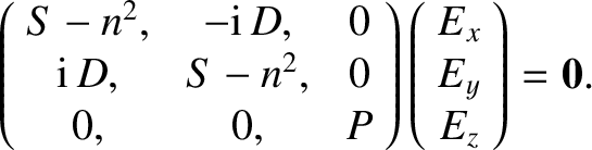
 , the eigenmode equation
(5.42) simplifies to
One obvious way of solving this equation is to have
, the eigenmode equation
(5.42) simplifies to
One obvious way of solving this equation is to have
 |
(5.89) |
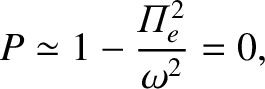
 . This is just the electrostatic plasma wave
that we found previously in an unmagnetized plasma. This mode is
longitudinal in nature, and, therefore, causes particles to
oscillate parallel to
. This is just the electrostatic plasma wave
that we found previously in an unmagnetized plasma. This mode is
longitudinal in nature, and, therefore, causes particles to
oscillate parallel to  . It follows that the particles
experience zero Lorentz force due to the presence of the equilibrium magnetic
field, with the result that this field has no effect on the mode dynamics.
. It follows that the particles
experience zero Lorentz force due to the presence of the equilibrium magnetic
field, with the result that this field has no effect on the mode dynamics.
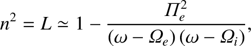
The other two solutions to Equation (5.88) are obtained by setting the  determinant involving the
  - and
- and  -components of the electric
field to zero. The first wave has the dispersion relation
-components of the electric
field to zero. The first wave has the dispersion relation
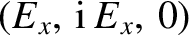 . This is evidently
a right-handed circularly polarized wave.
The second wave has the dispersion relation
and the eigenvector
. This is evidently
a right-handed circularly polarized wave.
The second wave has the dispersion relation
and the eigenvector
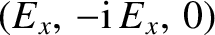 . This is evidently
a left-handed circularly polarized wave. At low frequencies
(i.e.,
. This is evidently
a left-handed circularly polarized wave. At low frequencies
(i.e.,
 ), both waves convert into the
Alfvén wave discussed in the previous section. (The fast and
slow Alfvén waves are indistinguishable for parallel
propagation.) Let us now examine the high-frequency behavior
of the right- and left-handed waves.
), both waves convert into the
Alfvén wave discussed in the previous section. (The fast and
slow Alfvén waves are indistinguishable for parallel
propagation.) Let us now examine the high-frequency behavior
of the right- and left-handed waves.
For the right-handed wave, because
 is
negative, it is evident that
is
negative, it is evident that
 as
as
 .
This resonance, which corresponds to
.
This resonance, which corresponds to
 ,
is termed the electron cyclotron resonance.
At the electron cyclotron resonance, the transverse electric field
associated with a right-handed
wave rotates at the same velocity, and in the same direction, as electrons
gyrating around the equilibrium magnetic field. Thus, the electrons
experience a continuous acceleration from the electric field, which tends
to increase their perpendicular energy. It is, therefore, not surprising that
right-handed waves, propagating
parallel to the equilibrium magnetic field,
and oscillating at the frequency
,
is termed the electron cyclotron resonance.
At the electron cyclotron resonance, the transverse electric field
associated with a right-handed
wave rotates at the same velocity, and in the same direction, as electrons
gyrating around the equilibrium magnetic field. Thus, the electrons
experience a continuous acceleration from the electric field, which tends
to increase their perpendicular energy. It is, therefore, not surprising that
right-handed waves, propagating
parallel to the equilibrium magnetic field,
and oscillating at the frequency
 , are absorbed by
electrons.
, are absorbed by
electrons.
When  lies just above
 , we find that
  is negative,
and so there is no wave propagation. However, for frequencies
much greater than the electron cyclotron or plasma frequencies, the solution
to Equation (5.90) is approximately
is negative,
and so there is no wave propagation. However, for frequencies
much greater than the electron cyclotron or plasma frequencies, the solution
to Equation (5.90) is approximately  . In other words,
 , which is the
dispersion relation of a right-handed vacuum electromagnetic wave.
Evidently, at some frequency above
, the solution
for must pass through zero, and become positive again.
Putting
, which is the
dispersion relation of a right-handed vacuum electromagnetic wave.
Evidently, at some frequency above
, the solution
for must pass through zero, and become positive again.
Putting  in Equation (5.90), we find that the equation reduces to
 |
(5.92) |
 . The previous equation has only
one positive root, at
. The previous equation has only
one positive root, at
 , where
Above this frequency, the wave propagates once again.
, where
Above this frequency, the wave propagates once again.
![\includegraphics[height=3in]{Chapter05/fig5_1.eps}](img1844.png) |
The dispersion curve for a right-handed wave propagating parallel to
the equilibrium
magnetic field is sketched in Figure 5.1. The continuation of the Alfvén
wave above the ion cyclotron frequency is called the electron cyclotron
wave, or, sometimes, the whistler wave. The latter terminology is prevalent
in ionospheric and space plasma physics contexts. The wave that propagates
above the cutoff frequency,  , is a standard right-handed
circularly polarized electromagnetic wave, somewhat modified by the
presence of the plasma. The low-frequency branch of the
dispersion curve differs fundamentally from the high-frequency branch, because
the former branch corresponds to a wave that can only propagate through the
plasma in the presence of an equilibrium magnetic field, whereas the latter
branch corresponds to a wave that can propagate in the absence of an equilibrium
field.
, is a standard right-handed
circularly polarized electromagnetic wave, somewhat modified by the
presence of the plasma. The low-frequency branch of the
dispersion curve differs fundamentally from the high-frequency branch, because
the former branch corresponds to a wave that can only propagate through the
plasma in the presence of an equilibrium magnetic field, whereas the latter
branch corresponds to a wave that can propagate in the absence of an equilibrium
field.
The curious name “whistler wave” for the branch of the dispersion relation lying between the ion and electron cyclotron frequencies is originally derived from ionospheric physics. Whistler waves are a very characteristic type of audio-frequency radio interference, most commonly encountered at high latitudes, which take the form of brief, intermittent pulses, starting at high frequencies, and rapidly descending in pitch.
Whistlers were discovered in the early days of radio communication, but
were not explained until much later (Storey 1953). Whistler waves start off as “instantaneous”
radio
pulses, generated by lightning flashes at high latitudes. The pulses are
channeled along the Earth's dipolar magnetic field, and eventually return
to ground level in the opposite hemisphere. Now, in the frequency
range
 , the dispersion
relation (5.90) reduces to
, the dispersion
relation (5.90) reduces to
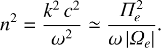 |
(5.94) |
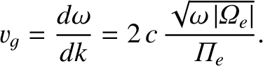 |
(5.95) |
The shape of whistler pulses, and the way in which the pulse frequency varies in time, can yield a considerable amount of information about the regions of the Earth's magnetosphere through which the pulses have passed. For this reason, many countries maintain observatories in polar regions—especially Antarctica—which monitor and collect whistler data.
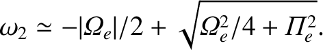
For a left-handed circularly polarized wave, similar considerations
to those described previously yield a dispersion
curve of the form sketched in Figure 5.2. In this case, goes to
infinity at the ion cyclotron frequency,
 , corresponding to
the so-called ion cyclotron resonance (at
, corresponding to
the so-called ion cyclotron resonance (at
 ). At this resonance, the
rotating electric
field associated with a left-handed wave resonates with the gyromotion
of the ions, allowing wave energy to be converted into perpendicular kinetic
energy of the ions. There is a band of frequencies, lying above the ion cyclotron
frequency, in which the left-handed wave does not propagate. At very high
frequencies, a propagating mode exists, which is basically a standard
left-handed circularly polarized electromagnetic wave, somewhat modified
by the presence of the plasma. The cutoff frequency for this wave is
). At this resonance, the
rotating electric
field associated with a left-handed wave resonates with the gyromotion
of the ions, allowing wave energy to be converted into perpendicular kinetic
energy of the ions. There is a band of frequencies, lying above the ion cyclotron
frequency, in which the left-handed wave does not propagate. At very high
frequencies, a propagating mode exists, which is basically a standard
left-handed circularly polarized electromagnetic wave, somewhat modified
by the presence of the plasma. The cutoff frequency for this wave is