Guiding Center Motion
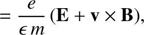
Consider the motion of a charged particle of mass  and charge
  in the limit in which
the electromagnetic fields experienced
by the particle do not vary much in a gyroperiod, so that
The electric force is assumed to be comparable to the magnetic force.
To keep track of the order of the various quantities, we introduce the parameter
in the limit in which
the electromagnetic fields experienced
by the particle do not vary much in a gyroperiod, so that
The electric force is assumed to be comparable to the magnetic force.
To keep track of the order of the various quantities, we introduce the parameter
 as a book-keeping device, and make the substitution
 , as well as
 . The parameter
is set to unity in the final answer.
. The parameter
is set to unity in the final answer.
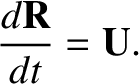
In order to make use of the technique described in the previous section, we write the
dynamical equations in the first-order differential form,
and seek a change of variables (Hazeltine and Waelbroeck 2004),
such that the new guiding center variables  and
and  are
free of oscillations along the particle trajectory. Here,
are
free of oscillations along the particle trajectory. Here,  is a
new independent variable describing the phase of the gyrating particle.
The functions
is a
new independent variable describing the phase of the gyrating particle.
The functions
 and
and  represent the gyration radius
and velocity, respectively. We require periodicity of these functions
with respect to their last argument, with period
represent the gyration radius
and velocity, respectively. We require periodicity of these functions
with respect to their last argument, with period  , and with vanishing mean, so that
Here, the angular brackets refer to the average over a period in .
, and with vanishing mean, so that
Here, the angular brackets refer to the average over a period in .
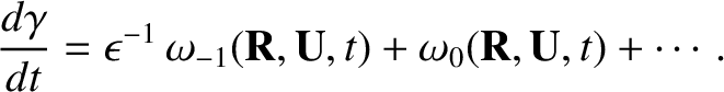
The equation of motion is used to determine the coefficients in the following expansion
of
and (Hazeltine and Waelbroeck 2004):
The dynamical equation for the gyrophase is likewise expanded,
assuming that
 ,
,
 |
(2.30) |
In the following, we suppress the subscripts on all quantities except
the guiding center velocity , because this is the only quantity for
which the first-order corrections are calculated.
To each order in , the evolution of the guiding center position,
, and velocity, ,
are determined by
the solubility conditions for the equations of motion, Equations (2.23) and (2.24), when
expanded to that order.
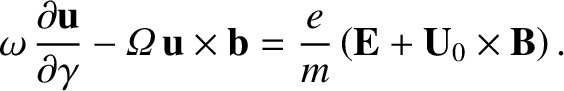
The oscillating components of the equations of motion determine the
evolution of the gyrophase. The velocity equation,
Equation (2.23), is linear. It follows that, to all orders in , its solubility condition is simply
 |
(2.31) |
To lowest order [that is,
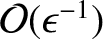 ], the momentum equation, Equation (2.24), yields
 |
(2.32) |
The solubility condition (that is, the gyrophase average) is
 |
(2.33) |
This immediately implies that
 |
(2.34) |
In other words, the rapid acceleration caused by a large parallel electric
field would invalidate the ordering assumptions used in this calculation.
Solving for  , we obtain
 |
(2.35) |
where all quantities are evaluated at the guiding center position, . The
perpendicular component of the velocity,  , has the
same form—namely, Equation (2.4)—as that obtained for uniform fields. The parallel velocity,
, has the
same form—namely, Equation (2.4)—as that obtained for uniform fields. The parallel velocity,
 , is
undetermined at this order.
, is
undetermined at this order.
The integral of the oscillating component of Equation (2.32) yields
![$\displaystyle {\bf u} = {\bf c} + u_\perp \left[\sin \,({\mit\Omega}\,\gamma/\omega) \,{\bf e}_1
+\cos\,({\mit\Omega}\,\gamma/\omega)\,{\bf e}_2\right],$](img302.png) |
(2.36) |
where  is a constant vector, and
  and
and  are again
mutually
orthogonal unit vectors perpendicular to
are again
mutually
orthogonal unit vectors perpendicular to  . All quantities in the
previous equation are functions of , , and
. All quantities in the
previous equation are functions of , , and  .
The periodicity
constraint, combined with Equation (2.27), requires that
.
The periodicity
constraint, combined with Equation (2.27), requires that
 and
and
 . The gyration velocity is thus
 |
(2.37) |
and, from Equation (2.30), the gyrophase is given by
 |
(2.38) |
where  is the initial gyrophase. The amplitude,
  ,
of the gyration velocity is undetermined at this order.
,
of the gyration velocity is undetermined at this order.
The lowest order oscillating component of the velocity equation, Equation (2.23), yields
 |
(2.39) |
This is readily integrated to give
  |
(2.40) |
where
 . It follows that
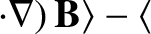
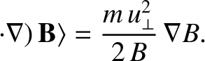
The gyrophase average of the first-order [that is,
 ]
momentum equation, Equation (2.24), reduces to
]
momentum equation, Equation (2.24), reduces to
![$\displaystyle \frac{d{\bf U}_0}{dt} = \frac{e}{m}\left[ E_\parallel\,{\bf b}
+ ...
...langle{\bf u}\times(\mbox{\boldmath$\rho$}\cdot\nabla)
\,{\bf B}\rangle\right].$](img316.png) |
(2.42) |
All quantities in the previous expression are functions of the
guiding center position, , rather than the instantaneous particle
position,  .
In order to evaluate the last term, we make the substitution
.
In order to evaluate the last term, we make the substitution

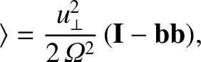
 , and calculate
The averages are specified by
where
, and calculate
The averages are specified by
where  is the identity tensor. Thus, making use of
 , it follows
that
This quantity is the secular component of the gyration induced fluctuations in the magnetic
force acting on the particle.
, it follows
that
This quantity is the secular component of the gyration induced fluctuations in the magnetic
force acting on the particle.
The coefficient of  in the previous equation,
 |
(2.46) |
plays a central role in the theory of magnetized particle motion. We can
interpret this coefficient as a magnetic moment by drawing an analogy
between a gyrating particle and a current loop. The (vector) magnetic moment of
a plane current loop is simply
  |
(2.47) |
where  is the current,
  the area of the loop, and
  the
unit normal to the surface of the loop. For a circular loop of
radius
, lying in the
plane perpendicular to , and carrying the current
the
unit normal to the surface of the loop. For a circular loop of
radius
, lying in the
plane perpendicular to , and carrying the current
 ,
we find
,
we find
 |
(2.48) |
We shall demonstrate, in Section 2.6, that the (scalar) magnetic moment,  , is a
constant of the particle motion. Thus, the guiding center behaves
exactly like a particle with a conserved magnetic moment that
is always aligned with the magnetic field.
, is a
constant of the particle motion. Thus, the guiding center behaves
exactly like a particle with a conserved magnetic moment that
is always aligned with the magnetic field.
The first-order guiding center equation of motion, Equation (2.42), reduces to
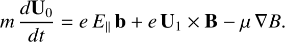 |
(2.49) |
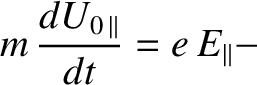
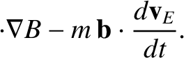
The component of this equation along the magnetic field determines the evolution
of the parallel guiding center velocity:
Here, use has been made of Equation (2.35), and
 .
The component of Equation (2.49) perpendicular to the magnetic field determines the
first-order perpendicular drift velocity:
.
The component of Equation (2.49) perpendicular to the magnetic field determines the
first-order perpendicular drift velocity:
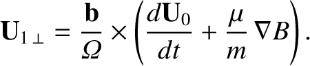 |
(2.51) |
The first-order correction to the parallel velocity, the so-called first-order parallel
drift velocity, is undetermined to this order. This is not a problem,
because the first-order parallel drift is a small correction to a type of motion
that already exists at zeroth order, whereas the first-order perpendicular drift is
a completely new type of motion. In particular, the first-order
perpendicular drift differs
fundamentally from the
 drift, because it is
not the same for all species, and, therefore, cannot be eliminated by transforming
to a new inertial frame. Thus, without loss of generality, we can absorb the first-order parallel drift into
, and write
drift, because it is
not the same for all species, and, therefore, cannot be eliminated by transforming
to a new inertial frame. Thus, without loss of generality, we can absorb the first-order parallel drift into
, and write
 .
.
We can now understand the motion of a charged particle as it moves through
slowly varying electric and magnetic fields. The particle always gyrates around
the magnetic field at the local gyrofrequency,
 .
The local perpendicular gyration velocity, , is determined by the
requirement that the magnetic moment,
.
The local perpendicular gyration velocity, , is determined by the
requirement that the magnetic moment,
 , be a
constant of the motion. This, in turn, fixes the local gyroradius,
.
The parallel velocity of the particle is determined by Equation (2.50).
Finally, the perpendicular drift velocity is the sum of the
drift velocity, , and the first-order drift velocity,
, be a
constant of the motion. This, in turn, fixes the local gyroradius,
.
The parallel velocity of the particle is determined by Equation (2.50).
Finally, the perpendicular drift velocity is the sum of the
drift velocity, , and the first-order drift velocity,