


Next: Magnetic Reconnection
Up: Magnetohydrodynamic Fluids
Previous: Cowling Anti-Dynamo Theorem
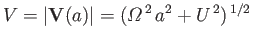
The simplest known kinematic dynamo is that
of Ponomarenko (Ponomarenko 1973). Consider a conducting fluid
of resistivity  that fills all space. The motion of the fluid
is confined to a cylinder of radius
that fills all space. The motion of the fluid
is confined to a cylinder of radius  . Adopting standard cylindrical coordinates
 aligned with this cylinder, the flow field is written
![$\displaystyle {\bf V} =\left\{ \begin{array}{lll} (0,\,r\,{\mit\Omega}, \,U)&\m...
... \mbox{for $r\leq a$}\\ [0.5ex] {\bf0} && \mbox{for $r>a$} \end{array} \right.,$](img2555.png) |
(7.139) |
where
 and
and  are constants. Note that the flow is
incompressible. In other words,
are constants. Note that the flow is
incompressible. In other words,
 .
.
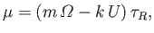
The MHD kinematic dynamo equation, (7.113), can be written
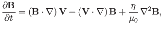 |
(7.140) |
where use has been made of
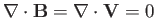 .
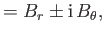
Let us search for solutions to this equation of the form
.
Let us search for solutions to this equation of the form
![$\displaystyle {\bf B}(r,\theta,z,t) = {\bf B}(r)\,\exp[\,{\rm i}\,(m\,\theta -k\, z)+\gamma\,t].$](img2558.png) |
(7.141) |
The  - and
- and  -components of Equation (7.140) are written (Huba 2000a)
and
respectively. In general, the term involving
 is zero. In fact, this term is only included in the analysis to enable
us to evaluate the correct matching conditions at
is zero. In fact, this term is only included in the analysis to enable
us to evaluate the correct matching conditions at  . We do not need to
write the
. We do not need to
write the  -component of Equation (7.140), because
  can be obtained
more directly from
can be obtained
more directly from  and
and  via the constraint
 .
.
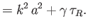
Let
 |
 |
(7.144) |
 |
 |
(7.145) |
 |
 |
(7.146) |
 |
 |
(7.147) |
 |
 |
(7.148) |
Here,  is the typical time required for magnetic flux to diffuse a distance
under the action of resistivity. Equations (7.142)-(7.148) can be
combined to give
is the typical time required for magnetic flux to diffuse a distance
under the action of resistivity. Equations (7.142)-(7.148) can be
combined to give
![$\displaystyle y^2\,\frac{d^2 B_\pm}{dy^2} + y\,\frac{d B_\pm}{dy} -\left[(m\pm 1)^2 + q^2\,y^2\right]B_\pm = 0$](img2578.png) |
(7.149) |
for  , and
, and
![$\displaystyle y^2\,\frac{d^2 B_\pm}{dy^2} + y\,\frac{d B_\pm}{dy} -\left[(m\pm 1)^2 + s^2\,y^2\right]B_\pm = 0$](img2580.png) |
(7.150) |
for  . The previous equations are modified
Bessel's equations of order
. The previous equations are modified
Bessel's equations of order  (Abramowitz and Stegun 1965b).
Thus, the physical solutions of Equations (7.149) and (7.150) that are well behaved
as
(Abramowitz and Stegun 1965b).
Thus, the physical solutions of Equations (7.149) and (7.150) that are well behaved
as
 and
and
 can be written
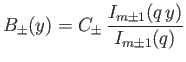 |
(7.151) |
for
, and
 |
(7.152) |
for
. Here,  and
and  are arbitrary constants.
Note that the arguments of
are arbitrary constants.
Note that the arguments of  and
and  are both constrained to lie in the
range
are both constrained to lie in the
range  to
to  .
.
The first matching condition at  is the continuity of
  , which yields
 |
(7.153) |
The second matching condition is obtained by integrating Equation (7.143)
from
 to
, where
to
, where  is an infinitesimal
quantity, and making use of the fact that the angular velocity
jumps discontinuously to zero at
. It follows that
is an infinitesimal
quantity, and making use of the fact that the angular velocity
jumps discontinuously to zero at
. It follows that
![$\displaystyle a\,{\mit\Omega}\,B_r = \frac{\eta}{\mu_0} \left[\frac{d B_\theta}{dr}\right]_{r=a_-}^{r=a_+}.$](img2593.png) |
(7.154) |
Furthermore, integration of Equation (7.142) tells us that  is continuous
at
. We can combine this information to give the matching
condition
is continuous
at
. We can combine this information to give the matching
condition
![$\displaystyle \left[\frac{d B_\pm}{dy}\right]_{y=1_-}^{y=1_+} =\pm{\rm i}\,{\mit\Omega}\,\tau_R\left( \frac{B_+ +B_-}{2}\right).$](img2595.png) |
(7.155) |
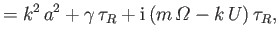
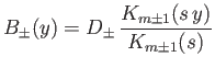
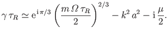
Equations (7.151)-(7.155) yield the dispersion relation
 |
(7.156) |
where
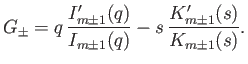 |
(7.157) |
Here,  denotes a derivative with respect to argument.
Unfortunately, despite the fact that we are investigating the simplest known kinematic dynamo,
the dispersion relation (7.156) is sufficiently complicated that it can only
be solved numerically. We can simplify matters considerably
taking the limit
 , which corresponds
to that of small wavelength (i.e.,
, which corresponds
to that of small wavelength (i.e.,  ).
The large argument asymptotic behavior of the Bessel functions is
specified by (Abramowitz and Stegun 1965b)
).
The large argument asymptotic behavior of the Bessel functions is
specified by (Abramowitz and Stegun 1965b)
where
 .
It follows that
.
It follows that
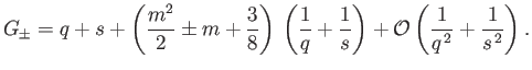 |
(7.160) |
Thus, the dispersion relation (7.156) reduces to
 |
(7.161) |
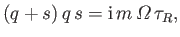
where  ,
,
 .
.
In the limit
 , where
 |
(7.162) |
which corresponds to
 , the simplified dispersion
relation (7.161) can be solved to give
, the simplified dispersion
relation (7.161) can be solved to give
 |
(7.163) |
Dynamo behavior [i.e.,
 ] takes place
when
] takes place
when
 |
(7.164) |
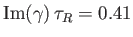
Observe that
 , implying that the
dynamo mode oscillates, or rotates, as well as growing exponentially in time.
The dynamo generated magnetic field is both non-axisymmetric [note that
dynamo activity is impossible, according to Equation (7.163), if
, implying that the
dynamo mode oscillates, or rotates, as well as growing exponentially in time.
The dynamo generated magnetic field is both non-axisymmetric [note that
dynamo activity is impossible, according to Equation (7.163), if  ] and
three-dimensional, and is, thus, not subject to either of the anti-dynamo
theorems mentioned in the preceding section.
] and
three-dimensional, and is, thus, not subject to either of the anti-dynamo
theorems mentioned in the preceding section.
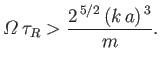
It is clear, from Equation (7.164), that dynamo action occurs whenever the flow
is made sufficiently rapid. But, what is the minimum amount of flow
needed to give rise to dynamo action?
In order to answer this question, we
have to solve the full dispersion relation, (7.156), for various values
of  and
and  , in order to find the dynamo mode that grows exponentially in time
for the smallest values of
and
. It is conventional
to parameterize the flow in terms of the magnetic Reynolds number,
, in order to find the dynamo mode that grows exponentially in time
for the smallest values of
and
. It is conventional
to parameterize the flow in terms of the magnetic Reynolds number,
 |
(7.165) |
where
 |
(7.166) |
is the typical timescale for convective motion across the system. Here,
 is a typical flow velocity, and
  is the characteristic lengthscale of the system.
Taking
is the characteristic lengthscale of the system.
Taking
 , and
, and  , we
have
, we
have
 |
(7.167) |
for the Ponomarenko dynamo. The critical value of the Reynolds number above
which dynamo action occurs is found to be (Ponomarenko 1973)
 |
(7.168) |
The most unstable dynamo mode is characterized by
 ,
,
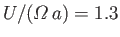 ,
,  ,
and
,
and
 . As the magnetic Reynolds number,
  ,
is increased above
the critical value,
,
is increased above
the critical value,  , other dynamo modes are eventually destabilized.
In 2000, the
Ponomarenko dynamo was realized experimentally by means of a tall cylinder filled with liquid sodium in which helical flow was excited
by a propeller (Gailitis et al. 2000). More information on laboratory dynamo experiments can be found in Verhille et alia 2009.
Next: Magnetic Reconnection
Up: Magnetohydrodynamic Fluids
Previous: Cowling Anti-Dynamo Theorem
Richard Fitzpatrick
2016-01-23
![$\displaystyle = {\rm e}^{\,-z}\left[1+\frac{4\,m^2-1}{8\,z} +{\cal O}\left(\frac{1}{z^2}\right)\right],$](img2602.png)
![$\displaystyle = {\rm e}^{\,+z}\left[1-\frac{4\,m^2-1}{8\,z} +{\cal O}\left(\frac{1}{z^2}\right)\right],$](img2604.png)
![$\displaystyle \phantom{=}+ \frac{\eta}{\mu_0} \left[\frac{d^2 B_r}{dr^{\,2}} + ...
...k^2 r^{\,2} +1)\,B_r}{r^{\,2}}- \frac{{\rm i}\,2\,m\,B_\theta}{r^{\,2}}\right],$](img2561.png)
![$\displaystyle \phantom{=}+ \frac{\eta}{\mu_0} \left[\frac{d^2 B_\theta}{dr^{\,2...
...k^2 r^{\,2} +1)\,B_\theta}{r^{\,2}}+ \frac{{\rm i}\,2\,m\,B_r}{r^{\,2}}\right],$](img2564.png)