


Next: Interplanetary Magnetic Field
Up: Magnetohydrodynamic Fluids
Previous: Solar Wind
By symmetry, we expect a purely radial, steady-state, coronal outflow.
The radial equation of motion of the corona [which is a modified version of Equation (7.2)] takes the form (Huba 2000b)
 |
(7.61) |
where  is the radial expansion speed.
The continuity equation [which is equivalent to Equation (7.1)] reduces to (Huba 2000b)
is the radial expansion speed.
The continuity equation [which is equivalent to Equation (7.1)] reduces to (Huba 2000b)
 |
(7.62) |
In order to obtain a closed set of equations, we now need to adopt an equation
of state for the corona, relating the pressure,  , and the density,
  . For
the sake of simplicity, we adopt the simplest conceivable equation
of state, which corresponds to an isothermal corona. Thus,
we have
. For
the sake of simplicity, we adopt the simplest conceivable equation
of state, which corresponds to an isothermal corona. Thus,
we have
 |
(7.63) |
where  is a constant. More realistic
equations of state complicate the analysis, but do not significantly modify
any of the physics results (Priest 1984).
is a constant. More realistic
equations of state complicate the analysis, but do not significantly modify
any of the physics results (Priest 1984).
Equation (7.62) can be integrated to give
 |
(7.64) |
where  is a constant. The previous expression simply states that the mass flux per
unit solid angle, which takes the value
, is independent of the radius,
is a constant. The previous expression simply states that the mass flux per
unit solid angle, which takes the value
, is independent of the radius,  .
Equations (7.61), (7.63), and (7.64) can be combined to give
.
Equations (7.61), (7.63), and (7.64) can be combined to give
 |
(7.65) |
Let us restrict our attention to coronal temperatures that satisfy
 |
(7.66) |
where  is the radius of the base of the corona. For typical
coronal parameters,
is the radius of the base of the corona. For typical
coronal parameters,
 K, which
is certainly greater than the temperature of the corona at
K, which
is certainly greater than the temperature of the corona at  . For
. For
 , the right-hand side of Equation (7.65) is negative for
 , where
 |
(7.67) |
and positive for
 . The right-hand side of (7.65) is zero at
 , implying that the left-hand side is also zero
at this radius, which is usually termed the ``critical radius.''
There are two ways in which the left-hand side of (7.65) can be zero at the critical
radius. Either
, implying that the left-hand side is also zero
at this radius, which is usually termed the ``critical radius.''
There are two ways in which the left-hand side of (7.65) can be zero at the critical
radius. Either
 |
(7.68) |
or
 |
(7.69) |
Note that  is the coronal sound speed.
As is easily demonstrated, if Equation (7.68) is satisfied then  has the
same sign for all
, and
has the
same sign for all
, and  is either a monotonically
increasing, or a monotonically decreasing, function of
. On the other
hand, if Equation (7.69) is satisfied then
is either a monotonically
increasing, or a monotonically decreasing, function of
. On the other
hand, if Equation (7.69) is satisfied then
 has the same
sign for all
, and
has an extremum close to
. The flow
is either super-sonic for all
, or sub-sonic for all
. These
possibilities lead to the existence of four classes of solutions
to Equation (7.65), with the
following properties:
has the same
sign for all
, and
has an extremum close to
. The flow
is either super-sonic for all
, or sub-sonic for all
. These
possibilities lead to the existence of four classes of solutions
to Equation (7.65), with the
following properties:
-
is sub-sonic throughout the domain
 .
increases with
, attains a maximum value around
, and then
decreases with
.
.
increases with
, attains a maximum value around
, and then
decreases with
.
- a unique solution for which
increases monotonically
with
, and
 .
.
- a unique solution for which
decreases monotonically
with
, and
.
-
is super-sonic throughout the domain
.
decreases with
, attains a minimum value around
, and then
increases with
.
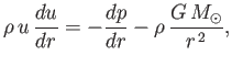
These four classes of solutions are illustrated in Figure 7.2.
Figure 7.2:
The four classes of Parker outflow solutions for the solar wind.
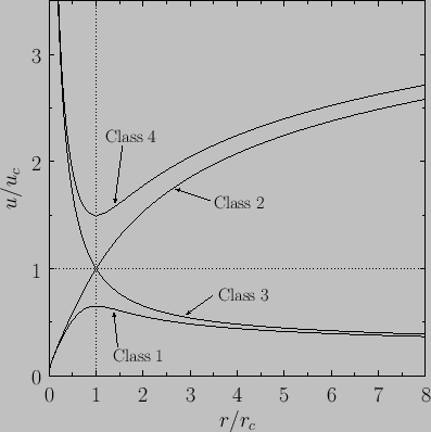 |
Each of the classes of solutions described previously fits a different
set of boundary conditions at
and
 . The
physical acceptability of these solutions depends on these
boundary conditions. For example, both Class 3 and Class 4 solutions can
be ruled out as plausible models for the solar corona because they predict
super-sonic flow at the base of the corona, which is not observed, and is
also not consistent with a static solar photosphere. Class 1 and Class 2 solutions
remain acceptable models for the solar corona on the basis of their
properties around
, because they both predict sub-sonic flow in this region.
However, the Class 1 and Class 2 solutions behave quite differently
as
, and the physical acceptability of these two
classes hinges on this difference.
. The
physical acceptability of these solutions depends on these
boundary conditions. For example, both Class 3 and Class 4 solutions can
be ruled out as plausible models for the solar corona because they predict
super-sonic flow at the base of the corona, which is not observed, and is
also not consistent with a static solar photosphere. Class 1 and Class 2 solutions
remain acceptable models for the solar corona on the basis of their
properties around
, because they both predict sub-sonic flow in this region.
However, the Class 1 and Class 2 solutions behave quite differently
as
, and the physical acceptability of these two
classes hinges on this difference.
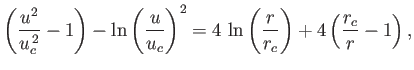
Equation (7.65) can be rearranged to give
 |
(7.70) |
where use has been made of Equations (7.66) and (7.67).
The previous expression can be integrated to give
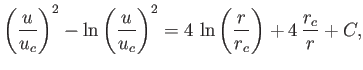 |
(7.71) |
where  is a constant of integration.
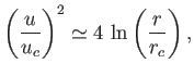
Let us consider the behavior
of Class 1 solutions in the limit
. It is
clear from Figure 7.2 that, for Class 1 solutions,  is less than unity and monotonically
decreasing as
. In the large-
limit, Equation (7.71)
reduces to
is less than unity and monotonically
decreasing as
. In the large-
limit, Equation (7.71)
reduces to
 |
(7.72) |
so that
 |
(7.73) |
It follows from Equation (7.64) that the coronal density,
, approaches
a finite, constant value,
 , as
. Thus,
the Class 1 solutions yield a finite pressure,
, as
. Thus,
the Class 1 solutions yield a finite pressure,
 |
(7.74) |
at large
, which cannot be matched to the much smaller pressure of the
interstellar medium. Obviously, Class 1 solutions are unphysical.
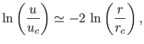
Let us consider the behavior of the Class 2 solution
in the limit
. It is
clear from Figure 7.2 that, for the Class 2 solution,
is greater than unity and monotonically
increasing as
. In the large-
limit,
Equation (7.71) reduces to
 |
(7.75) |
so that
![$\displaystyle u \simeq 2\,u_c\left[\ln\left(\frac{r}{r_c}\right)\right]^{\,1/2}.$](img2380.png) |
(7.76) |
It follows from Equation (7.64) that
 as
. Thus, the Class 2 solution yields
as
. Thus, the Class 2 solution yields
 at large
, and can, therefore, be matched to the low
pressure interstellar medium.
at large
, and can, therefore, be matched to the low
pressure interstellar medium.
We conclude that the only solution to Equation (7.65) that is consistent
with the physical boundary conditions at
and
is
the Class 2 solution. This solution predicts that the
solar corona expands radially outward at
relatively modest, sub-sonic velocities close to the Sun,
and gradually accelerates
to super-sonic velocities as it moves further away from the Sun.
Parker termed this continuous, super-sonic expansion of the corona
the ``solar wind.''
Equation (7.71) can be rewritten
 |
(7.77) |
where the constant
is determined by demanding that
 when
. Note that both
and
when
. Note that both
and  can be evaluated
in terms of the coronal temperature,
, via Equations (7.67) and (7.68).
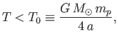
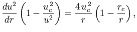
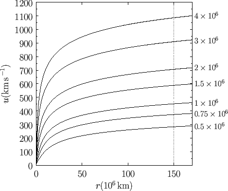
Figure 7.3 shows
calculated from Equation (7.77) for various values
of the coronal temperature. It can be seen that plausible
values of
(i.e.,
can be evaluated
in terms of the coronal temperature,
, via Equations (7.67) and (7.68).
Figure 7.3 shows
calculated from Equation (7.77) for various values
of the coronal temperature. It can be seen that plausible
values of
(i.e.,  -
-
 K) yield
expansion speeds of several hundreds of kilometers per second
at 1 AU, which accords well with satellite observations. The critical
surface where the solar wind makes the transition from sub-sonic to
super-sonic flow is predicted to lie a few solar radii away from the Sun
(i.e.,
K) yield
expansion speeds of several hundreds of kilometers per second
at 1 AU, which accords well with satellite observations. The critical
surface where the solar wind makes the transition from sub-sonic to
super-sonic flow is predicted to lie a few solar radii away from the Sun
(i.e.,
 , where
  is the solar radius). Unfortunately, the Parker model's
prediction for the density of the solar wind at the Earth is significantly
too high compared to satellite observations. Consequently, there have
been many further developments of this model. In particular, the
unrealistic assumption that the solar wind plasma is isothermal has been relaxed, and
two-fluid effects have been incorporated into the analysis (Priest 1984).
is the solar radius). Unfortunately, the Parker model's
prediction for the density of the solar wind at the Earth is significantly
too high compared to satellite observations. Consequently, there have
been many further developments of this model. In particular, the
unrealistic assumption that the solar wind plasma is isothermal has been relaxed, and
two-fluid effects have been incorporated into the analysis (Priest 1984).
Figure 7.3:
Parker outflow solutions for the solar wind. Each curve is labelled by the corresponding coronal
temperature in degrees kelvin. The vertical dashed line indicates the mean radius of the Earth's orbit.
 |
Next: Interplanetary Magnetic Field
Up: Magnetohydrodynamic Fluids
Previous: Solar Wind
Richard Fitzpatrick
2016-01-23