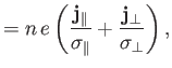
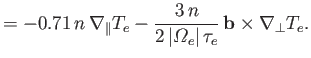
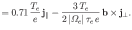
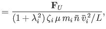
Let us consider a magnetized plasma. It is convenient to split the friction force
![]() into a component
into a component ![]() corresponding to resistivity, and a
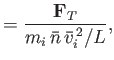
component
corresponding to resistivity, and a
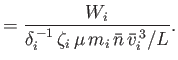
component ![]() corresponding to the thermal force. Thus,
corresponding to the thermal force. Thus,
| (4.138) |
 |
(4.139) | |
 |
(4.140) |
| (4.141) |
 |
(4.142) | |
 |
(4.143) |
| (4.144) |
| (4.145) | ||
 |
(4.146) |
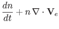
Let us, first of all, consider the electron fluid equations, which can be written:
 |
(4.147) | |
 |
(4.148) | |
 |
||
| (4.149) |
 |
(4.150) | |
 |
(4.151) | |
 |
(4.152) |
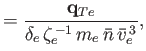
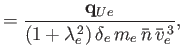
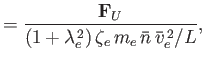
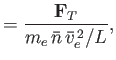
We define the following normalized quantities:
 |
||||||
 |
 |
|||||
 |
 |
|||||
 |
 |
 |
||||
 |
 |
 |
||||
 |
 |
 |
The normalization procedure is designed to make all hatted quantities
![]() .
The normalization of the electric field is chosen
such that the
.
The normalization of the electric field is chosen
such that the
![]() velocity is of similar magnitude to the electron fluid velocity. Note that the parallel viscosity
makes an
velocity is of similar magnitude to the electron fluid velocity. Note that the parallel viscosity
makes an
![]() contribution to
contribution to
![]() , whereas the gyroviscosity
makes an
, whereas the gyroviscosity
makes an
![]() contribution, and the perpendicular viscosity only
makes an
contribution, and the perpendicular viscosity only
makes an
![]() contribution. Likewise, the parallel thermal
conductivity
makes an
contribution. Likewise, the parallel thermal
conductivity
makes an
![]() contribution to
contribution to
![]() , whereas the cross
conductivity
makes an
, whereas the cross
conductivity
makes an
![]() contribution, and the perpendicular conductivity only
makes an
contribution, and the perpendicular conductivity only
makes an
![]() contribution. Similarly, the parallel components
of
contribution. Similarly, the parallel components
of ![]() and
and
![]() are
are
![]() , whereas the perpendicular
components are
, whereas the perpendicular
components are
![]() .
.
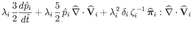
The normalized electron fluid equations take the form:
 |
(4.153) | |
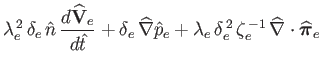 |
(4.154) | |
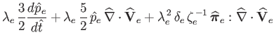 |
||
| (4.155) |
Let us now consider the ion fluid equations, which can be written:
 |
(4.156) | |
 |
(4.157) | |
 |
(4.158) |
| (4.159) | ||
| (4.160) | ||
|
(4.161) |
We define the following normalized quantities:
 |
 |
|||||
 |
 |
|||||
 |
 |
 |
||||
 |
 |
 |
As before, the normalization procedure is designed to make all hatted quantities
![]() .
The normalization of the electric field is chosen
such that the
.
The normalization of the electric field is chosen
such that the
![]() velocity is of similar magnitude to the ion fluid velocity. Note that the parallel viscosity
makes an
velocity is of similar magnitude to the ion fluid velocity. Note that the parallel viscosity
makes an
![]() contribution to
contribution to
![]() , whereas the gyroviscosity
makes an
, whereas the gyroviscosity
makes an
![]() contribution, and the perpendicular viscosity only
makes an
contribution, and the perpendicular viscosity only
makes an
![]() contribution. Likewise, the parallel thermal
conductivity
makes an
contribution. Likewise, the parallel thermal
conductivity
makes an
![]() contribution to
contribution to
![]() , whereas the cross
conductivity
makes an
, whereas the cross
conductivity
makes an
![]() contribution, and the perpendicular conductivity only
makes an
contribution, and the perpendicular conductivity only
makes an
![]() contribution. Similarly, the parallel component
of
contribution. Similarly, the parallel component
of ![]() is
is
![]() , whereas the perpendicular
component is
, whereas the perpendicular
component is
![]() .
.
The normalized ion fluid equations take the form:
 |
(4.162) | |
 |
(4.163) | |
 |
||
| (4.164) |
Let us adopt the ordering
| (4.165) |
| (4.166) | ||
| (4.167) | ||
| (4.168) | ||
| (4.169) | ||
| (4.170) |
There are three fundamental orderings in plasma fluid theory. These are analogous to the three orderings in neutral gas fluid theory discussed in Section 4.9.
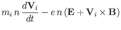
The first ordering is
Equations (4.174)-(4.175) and (4.176)-(4.177) are called the cold-plasma equations, because
they can be obtained from the Braginskii equations by formally taking the
limit
![]() . Likewise, the ordering (4.171) is called
the cold-plasma approximation. The cold-plasma approximation
applies not only to cold plasmas, but also to very fast disturbances that
propagate through conventional plasmas. In particular,
the cold-plasma equations provide a good description of the propagation
of electromagnetic waves through plasmas. After all, electromagnetic
waves generally have very high velocities (i.e.,
. Likewise, the ordering (4.171) is called
the cold-plasma approximation. The cold-plasma approximation
applies not only to cold plasmas, but also to very fast disturbances that
propagate through conventional plasmas. In particular,
the cold-plasma equations provide a good description of the propagation
of electromagnetic waves through plasmas. After all, electromagnetic
waves generally have very high velocities (i.e., ![]() ),
which they impart to
plasma fluid elements, so there is usually
no difficulty satisfying the inequality (4.172).
),
which they impart to
plasma fluid elements, so there is usually
no difficulty satisfying the inequality (4.172).
The electron and ion pressures can be neglected in the cold-plasma limit, because the thermal velocities are much smaller than the fluid velocities. It follows that there is no need for an electron or ion energy evolution equation. Furthermore, the motion of the plasma is so fast, in this limit, that relatively slow ``transport'' effects, such as viscosity and thermal conductivity, play no role in the cold-plasma fluid equations. In fact, the only collisional effect that appears in these equations is resistivity.
The second ordering is
| (4.179) |
Equations (4.180)-(4.182) and (4.183)-(4.184) are called the magnetohydrodynamical equations, or MHD equations, for short. Likewise, the ordering (4.178) is called the MHD approximation. The MHD equations are conventionally used to study macroscopic plasma instabilities possessing relatively fast growth-rates: for example, ``sausage'' modes and ``kink'' modes (Bateman 1978).
The electron and ion pressures cannot be neglected in the MHD limit, because the fluid velocities are similar in magnitude to the respective thermal velocities. Thus, electron and ion energy evolution equations are needed in this limit. However, MHD motion is sufficiently fast that ``transport'' effects, such as viscosity and thermal conductivity, are too slow to play a role in the MHD equations. In fact, the only collisional effects that appear in these equations are resistivity, the thermal force, and electron-ion collisional energy exchange.
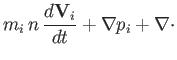
The final ordering is
| (4.187) |
|
(4.188) | |
![$\displaystyle m_e \,n\,\frac{d {\bf V}_e}{dt} + [\delta^{\,-2}]\,\nabla p_e+ [\zeta^{\,-1}]\, \nabla\cdot$](img1504.png) |
(4.189) | |
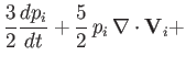
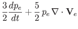
![$\displaystyle \frac{3}{2}\frac{d p_e}{dt} + \frac{5}{2}\,p_e\,\nabla\cdot{\bf V}_e + [\zeta^{\,-1}]\,\nabla\cdot{\bf q}_{Te} + \nabla\cdot{\bf q}_{Ue}$](img1508.png) |
||
| (4.190) |
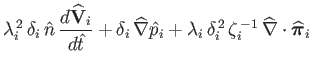
Equations (4.188)-(4.190) and (4.191)-(4.193) are called the drift equations. Likewise, the ordering (4.186) is called the drift approximation. The drift equations are conventionally used to study equilibrium evolution, and the slow growing ``micro-instabilities'' that are responsible for turbulent transport in tokamaks. It is clear that virtually all of the original terms in the Braginskii equations must be retained in this limit.
In the following sections, we investigate the cold-plasma equations, the MHD equations, and the drift equations, in more detail.

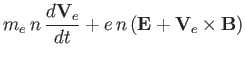
![$\displaystyle m_e \,n\,\frac{d {\bf V}_e}{dt} + \nabla p_e+ [\delta^{\,-1}]\,e\, n\, ({\bf E} + {\bf V}_e\times {\bf B})$](img1493.png)
![$\displaystyle m_i \,n\,\frac{d {\bf V}_i}{dt} + \nabla p_i - [\delta^{\,-1}]\, e \,n\, ({\bf E} + {\bf V}_i\times {\bf B})$](img1497.png)
![$\displaystyle m_i \,n\,\frac{d {\bf V}_i}{dt} + [\delta^{\,-2}]\,\nabla p_i + [\zeta^{\,-1}]\,\nabla\cdot$](img1511.png)
![$\displaystyle \frac{3}{2}\frac{d p_i}{dt} + \frac{5}{2}\,p_i\,\nabla\cdot{\bf V}_i + [\zeta^{\,-1}]\,\nabla\cdot{\bf q}_i$](img1515.png)