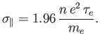
The first step in our closure scheme is to approximate the actual collision operator for Coulomb interactions by an operator that is strictly bilinear in its arguments. (See Section 3.10.) Once this has been achieved, the closure problem is formally of the type that can be solved using the Chapman-Enskog method.
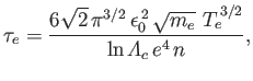
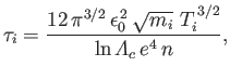
The electron-ion and ion-ion collision times are written
The basic forms of Equations (4.89) and (4.90) are not hard to understand. From Equation (4.58), we expect
 |
(4.91) |
 |
(4.92) |
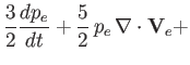
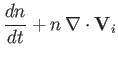
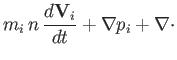
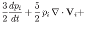
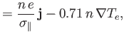
The electron and ion fluid equations in a collisional plasma take the form [see Equations (4.47)-(4.49)]:
In the unmagnetized limit, which actually corresponds to
| (4.99) |
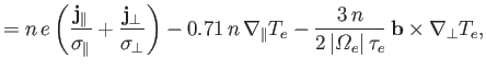
Let us examine each of the previous collisional terms, one by one. The first
term on the right-hand side of Equation (4.100) is a friction force caused by the
relative motion of electrons and ions, and obviously controls the electrical
conductivity of the plasma. The form of this term is fairly easy to understand.
The electrons lose their ordered velocity
with respect to the ions,
![]() ,
in an electron-ion collision time,
,
in an electron-ion collision time, ![]() , and consequently lose momentum
, and consequently lose momentum
![]() per electron (which is given to the ions) in this time.
This means that a frictional force
per electron (which is given to the ions) in this time.
This means that a frictional force
![]() is exerted on the electrons.
An equal and opposite force is exerted on the ions. Because the Coulomb
cross-section diminishes with increasing electron energy (i.e.,
is exerted on the electrons.
An equal and opposite force is exerted on the ions. Because the Coulomb
cross-section diminishes with increasing electron energy (i.e.,
![]() ),
the conductivity of the fast electrons in the distribution function
is higher than that of the slow electrons (because
),
the conductivity of the fast electrons in the distribution function
is higher than that of the slow electrons (because
![]() ).
Hence, electrical current in plasmas is carried predominately by the
fast electrons. This effect has some important and interesting
consequences.
).
Hence, electrical current in plasmas is carried predominately by the
fast electrons. This effect has some important and interesting
consequences.
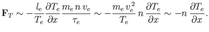
One immediate consequence is the second term on the right-hand side of Equation (4.100),
which is called the thermal force. To understand the origin of
a frictional force proportional to minus the gradient of the electron temperature,
let us assume that the electron and ion fluids are at rest (i.e.,
![]() ). It follows that the number of electrons moving from left to right
(along the
). It follows that the number of electrons moving from left to right
(along the ![]() -axis, say) and from right to left per unit time is exactly the
same at a given point (coordinate
-axis, say) and from right to left per unit time is exactly the
same at a given point (coordinate ![]() , say) in the plasma. As a result
of electron-ion collisions, these fluxes experience frictional forces,
, say) in the plasma. As a result
of electron-ion collisions, these fluxes experience frictional forces,
![]() and
and ![]() , respectively, of approximate magnitude
, respectively, of approximate magnitude
![]() ,
where
,
where ![]() is the electron thermal velocity. In a completely homogeneous
plasma, these forces balance exactly, and so there is zero net frictional force.
Suppose, however, that the electrons coming from the right are, on average, hotter
than those coming from the left. It follows that the frictional force
is the electron thermal velocity. In a completely homogeneous
plasma, these forces balance exactly, and so there is zero net frictional force.
Suppose, however, that the electrons coming from the right are, on average, hotter
than those coming from the left. It follows that the frictional force
![]() acting on the fast electrons coming from the right is less than
the force
acting on the fast electrons coming from the right is less than
the force ![]() acting on the slow electrons coming from the left, because
acting on the slow electrons coming from the left, because
![]() increases with electron temperature. As a result, there is a net
frictional force acting to the left: that is, in the direction of
increases with electron temperature. As a result, there is a net
frictional force acting to the left: that is, in the direction of
![]() .
.
Let us estimate the magnitude of the frictional force. At point ![]() , collisions
are experienced by electrons that have traversed distances of similar magnitude to a
mean-free-path,
, collisions
are experienced by electrons that have traversed distances of similar magnitude to a
mean-free-path,
![]() . Thus, the electrons coming from the
right originate from regions in which the temperature is approximately
. Thus, the electrons coming from the
right originate from regions in which the temperature is approximately
![]() greater than the regions from which the electrons
coming from the left originate. Because the friction force is proportional to
greater than the regions from which the electrons
coming from the left originate. Because the friction force is proportional to
![]() , the net force
, the net force
![]() is approximately
is approximately
The term ![]() , specified in Equation (4.101), represents the rate at which
energy is acquired by the ions due to collisions
with the electrons.
The most striking aspect of this term is
its smallness
(note that it is proportional to an inverse mass ratio,
, specified in Equation (4.101), represents the rate at which
energy is acquired by the ions due to collisions
with the electrons.
The most striking aspect of this term is
its smallness
(note that it is proportional to an inverse mass ratio,
![]() ). The smallness of
). The smallness of ![]() is a direct consequence of the
fact that electrons are considerably lighter than ions. Consider the
limit in which the ion mass is infinite, and the ions are at rest on average:
that is,
is a direct consequence of the
fact that electrons are considerably lighter than ions. Consider the
limit in which the ion mass is infinite, and the ions are at rest on average:
that is, ![]() . In this case, collisions of electrons with ions
take place without any exchange of energy. The electron velocities
are randomized by the collisions, so that the energy associated
with their ordered velocity,
. In this case, collisions of electrons with ions
take place without any exchange of energy. The electron velocities
are randomized by the collisions, so that the energy associated
with their ordered velocity,
![]() , is converted
into heat energy in the electron fluid [this is represented by the second term
on the extreme right-hand side of Equation (4.102)]. However, the ion energy remains
unchanged. Let us now assume that the ratio
, is converted
into heat energy in the electron fluid [this is represented by the second term
on the extreme right-hand side of Equation (4.102)]. However, the ion energy remains
unchanged. Let us now assume that the ratio ![]() is large, but finite, and
that
is large, but finite, and
that ![]() . If
. If ![]() then the ions and electrons are in thermal equilibrium, so
no heat is exchanged between them. However, if
then the ions and electrons are in thermal equilibrium, so
no heat is exchanged between them. However, if ![]() then heat
is transferred from the electrons to the ions. As is well known, when
a light particle collides with a heavy particle, the order of magnitude of the
transferred energy is given by the mass ratio
then heat
is transferred from the electrons to the ions. As is well known, when
a light particle collides with a heavy particle, the order of magnitude of the
transferred energy is given by the mass ratio ![]() , where
, where ![]() is the
mass of the lighter particle. For example, the mean fractional energy transferred
in isotropic scattering is
is the
mass of the lighter particle. For example, the mean fractional energy transferred
in isotropic scattering is
![]() . Thus, we would expect the
energy per unit time transferred from the electrons to the ions to be roughly
. Thus, we would expect the
energy per unit time transferred from the electrons to the ions to be roughly
 |
(4.105) |
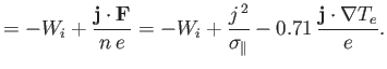
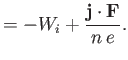
The term ![]() , specified in Equation (4.102), represents the rate at
which energy is acquired by the electrons because of
collisions with the ions, and consists of three terms. Not surprisingly,
the first term is simply minus the rate at which energy is
acquired by the ions due to collisions with the
electrons. The second term represents the conversion
of the ordered motion of the electrons, relative to the ions, into random
motion (i.e., heat) via collisions with the ions. This
term is positive definite, indicating that the randomization of the electron
ordered motion gives rise to irreversible heat generation.
Incidentally, this
term is usually called the ohmic heating term. Finally, the third
term represents the work done against the thermal force. This
term can be either positive or negative, depending on the direction of
the current flow relative to the electron temperature gradient, which
indicates that work done against the thermal force gives rise to reversible
heat generation. There is an analogous effect in metals called the Thomson effect (Doolittle 1959).
, specified in Equation (4.102), represents the rate at
which energy is acquired by the electrons because of
collisions with the ions, and consists of three terms. Not surprisingly,
the first term is simply minus the rate at which energy is
acquired by the ions due to collisions with the
electrons. The second term represents the conversion
of the ordered motion of the electrons, relative to the ions, into random
motion (i.e., heat) via collisions with the ions. This
term is positive definite, indicating that the randomization of the electron
ordered motion gives rise to irreversible heat generation.
Incidentally, this
term is usually called the ohmic heating term. Finally, the third
term represents the work done against the thermal force. This
term can be either positive or negative, depending on the direction of
the current flow relative to the electron temperature gradient, which
indicates that work done against the thermal force gives rise to reversible
heat generation. There is an analogous effect in metals called the Thomson effect (Doolittle 1959).
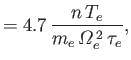
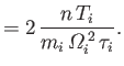
The electron and ion heat flux densities are given by
It follows, by comparison with Equations (4.63)-(4.68), that
the first term on the right-hand side of Equation (4.106), as well as the expression
on the right-hand side of Equation (4.107), represent straightforward
random-walk heat diffusion, with frequency ![]() , and step-length
, and step-length ![]() .
Recall, that
.
Recall, that
![]() is the collision frequency, and
is the collision frequency, and
![]() is the mean-free-path. The
electron heat diffusivity is generally much greater than that of the ions,
because
is the mean-free-path. The
electron heat diffusivity is generally much greater than that of the ions,
because
![]() ,
assuming that
,
assuming that
![]() .
.
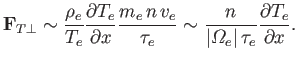
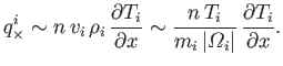
The second term on the right-hand side of Equation (4.106) describes a convective
heat flux due to the motion of the electrons relative to the ions.
To understand the origin of this flux, we need to recall that
electric current in plasmas is carried predominately by the fast electrons
in the distribution function. Suppose that ![]() is non-zero. In the
coordinate system in which
is non-zero. In the
coordinate system in which ![]() is zero, more fast electrons move in the
direction of
is zero, more fast electrons move in the
direction of ![]() , and more slow electrons move in the opposite
direction. Although the electron fluxes are balanced in this frame of reference,
the energy fluxes are not (because a fast electron possesses more energy than a slow
electron), and heat flows in the direction of
, and more slow electrons move in the opposite
direction. Although the electron fluxes are balanced in this frame of reference,
the energy fluxes are not (because a fast electron possesses more energy than a slow
electron), and heat flows in the direction of ![]() : that is, in
the opposite direction to the electric current. The net heat flux density is of
approximate magnitude
: that is, in
the opposite direction to the electric current. The net heat flux density is of
approximate magnitude ![]() , because there is no near cancellation of the fluxes
due to the fast and slow electrons. Like the thermal force, this effect
depends on collisions, despite the fact that the expression for the convective
heat flux does not contain
, because there is no near cancellation of the fluxes
due to the fast and slow electrons. Like the thermal force, this effect
depends on collisions, despite the fact that the expression for the convective
heat flux does not contain ![]() explicitly.
explicitly.
Finally, the electron and ion viscosity tensors take the form
Let us now examine the magnetized limit,
| (4.114) |
 |
(4.115) | |
 |
(4.116) | |
 |
(4.117) |
We expect the presence of a strong magnetic field to give rise to a
marked anisotropy in plasma properties between directions parallel
and perpendicular to ![]() , because of the completely different motions
of the constituent ions and electrons parallel and perpendicular to the field.
Thus, not surprisingly, we find that the electrical conductivity perpendicular
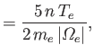
to the field is approximately half that parallel to the field [see Equations (4.115)
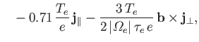
and (4.118)]. The thermal force is unchanged (relative to the unmagnetized case)
in the parallel direction, but is radically modified in the
perpendicular direction. In order to understand the origin
of the last term in Equation (4.115), let us consider a situation in
which there is a strong magnetic field along the
, because of the completely different motions
of the constituent ions and electrons parallel and perpendicular to the field.
Thus, not surprisingly, we find that the electrical conductivity perpendicular
to the field is approximately half that parallel to the field [see Equations (4.115)
and (4.118)]. The thermal force is unchanged (relative to the unmagnetized case)
in the parallel direction, but is radically modified in the
perpendicular direction. In order to understand the origin
of the last term in Equation (4.115), let us consider a situation in
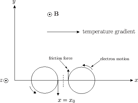
which there is a strong magnetic field along the ![]() -axis, and an electron
temperature gradient along the
-axis, and an electron
temperature gradient along the ![]() -axis. (See Figure 4.1.) The electrons gyrate
in the
-axis. (See Figure 4.1.) The electrons gyrate
in the ![]() -
-![]() plane in circles of radius
plane in circles of radius
![]() .
At a given point, coordinate
.
At a given point, coordinate ![]() , say, on the
, say, on the ![]() -axis, the electrons that
come from the right and the left have traversed distances of approximate magnitude
-axis, the electrons that
come from the right and the left have traversed distances of approximate magnitude ![]() .
Thus, the electrons from the right originate from regions where the
electron temperature is approximately
.
Thus, the electrons from the right originate from regions where the
electron temperature is approximately
![]() greater than
the regions from which the electrons from the left originate. Because the
friction force is proportional to
greater than
the regions from which the electrons from the left originate. Because the
friction force is proportional to
![]() , an unbalanced friction force
arises, directed along the
, an unbalanced friction force
arises, directed along the ![]() -axis. (See Figure 4.1.) This direction
corresponds to the direction of
-axis. (See Figure 4.1.) This direction
corresponds to the direction of
![]() .
There is
no friction force along the
.
There is
no friction force along the ![]() -axis, because the
-axis, because the ![]() -directed fluxes are associated with electrons that originate from regions where
-directed fluxes are associated with electrons that originate from regions where ![]() .
By analogy with Equation (4.104), the magnitude of the perpendicular
thermal force is
.
By analogy with Equation (4.104), the magnitude of the perpendicular
thermal force is
 |
(4.119) |
In the magnetized limit, the electron and ion heat flux densities become
 |
(4.122) | |
 |
(4.123) |
 |
(4.124) | |
 |
(4.125) |
The first two terms on the right-hand sides of Equations (4.120) and (4.121)
correspond to diffusive heat transport by the electron and ion
fluids, respectively. According to the first terms, the diffusive transport in
the direction parallel to the magnetic field is exactly the same as that in the
unmagnetized case: that is, it corresponds to
collision-induced random-walk diffusion
of the ions and electrons, with
frequency ![]() , and step-length
, and step-length ![]() . According to the
second terms, the diffusive transport in the direction perpendicular to the
magnetic field is far smaller than that in the parallel direction.
To be more exact, it is smaller by a factor
. According to the
second terms, the diffusive transport in the direction perpendicular to the
magnetic field is far smaller than that in the parallel direction.
To be more exact, it is smaller by a factor
![]() , where
, where ![]() is the
gyroradius, and
is the
gyroradius, and ![]() the mean-free-path. In fact, the perpendicular
heat transport also corresponds to collision-induced random-walk diffusion
of charged particles,
but with frequency
the mean-free-path. In fact, the perpendicular
heat transport also corresponds to collision-induced random-walk diffusion
of charged particles,
but with frequency ![]() , and
step-length
, and
step-length ![]() . Thus, it is the greatly reduced step-length in the
perpendicular direction, relative to the parallel direction, that ultimately
gives rise to the strong reduction in the perpendicular heat transport.
If
. Thus, it is the greatly reduced step-length in the
perpendicular direction, relative to the parallel direction, that ultimately
gives rise to the strong reduction in the perpendicular heat transport.
If
![]() then the ion perpendicular heat diffusivity actually
exceeds that of the electrons by the square root of a mass ratio: that is,
then the ion perpendicular heat diffusivity actually
exceeds that of the electrons by the square root of a mass ratio: that is,
![]() .
.
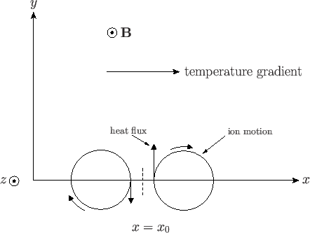
The third terms on the right-hand sides of Equations (4.120) and (4.121)
correspond to heat fluxes that are perpendicular to both the magnetic field
and the direction of the temperature gradient. In order to understand the
origin of these terms, let us consider the ion flux. Suppose that there
is a strong magnetic field along the ![]() -axis, and an ion temperature gradient
along the
-axis, and an ion temperature gradient
along the ![]() -axis. (See Figure 4.2.) The ions gyrate in the
-axis. (See Figure 4.2.) The ions gyrate in the ![]() -
-![]() plane
in circles of radius
plane
in circles of radius
![]() , where
, where ![]() is the
ion thermal velocity. At a given point, coordinate
is the
ion thermal velocity. At a given point, coordinate ![]() , say, on the
, say, on the ![]() -axis,
the ions that come from the right and the left have traversed distances of
approximate magnitude
-axis,
the ions that come from the right and the left have traversed distances of
approximate magnitude ![]() . The ions from the right are clearly somewhat hotter than those
from the left. If the unidirectional particle fluxes, of approximate magnitude
. The ions from the right are clearly somewhat hotter than those
from the left. If the unidirectional particle fluxes, of approximate magnitude ![]() , are
balanced, then the unidirectional heat fluxes, of approximate magnitude
, are
balanced, then the unidirectional heat fluxes, of approximate magnitude
![]() , will
have an unbalanced component of relative magnitude
, will
have an unbalanced component of relative magnitude
![]() . As a result, there is a net heat flux in the
. As a result, there is a net heat flux in the ![]() -direction
(i.e., the direction of
-direction
(i.e., the direction of
![]() ). The magnitude of
this flux is
). The magnitude of
this flux is
 |
(4.126) |
The fourth and fifth terms on the right-hand side of Equation (4.120) correspond to
the convective component of the electron heat flux density, driven by
motion of the electrons relative to the ions. It is clear from the
fourth term that the convective flux parallel to the magnetic field is exactly the
same as in the unmagnetized case [see Equation (4.106)]. However, according to the fifth term, the
convective flux is radically modified in the perpendicular direction.
Probably the easiest method of explaining the fifth
term is via an examination
of Equations (4.100), (4.106), (4.115), and (4.120). There is clearly a very close
connection between the electron thermal force and the convective heat flux.
In fact, starting from general principles of the thermodynamics of irreversible
processes--the so-called Onsager principles (Reif 1965)--it is possible to
demonstrate that an electron frictional force of the form
![]() necessarily gives rise to an electron heat flux
of the form
necessarily gives rise to an electron heat flux
of the form
![]() , where the
subscript
, where the
subscript ![]() corresponds to a general Cartesian component, and
corresponds to a general Cartesian component, and ![]() is a unit vector. Thus, the fifth term on the right-hand side of Equation (4.120)
follows by Onsager symmetry from the third term on the right-hand
side of Equation (4.115). This is one of many Onsager symmetries that
occur in plasma transport theory.
is a unit vector. Thus, the fifth term on the right-hand side of Equation (4.120)
follows by Onsager symmetry from the third term on the right-hand
side of Equation (4.115). This is one of many Onsager symmetries that
occur in plasma transport theory.
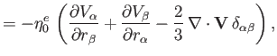
In order to describe the viscosity tensor in a magnetized plasma, it is helpful to define the rate-of-strain tensor
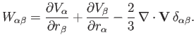 |
(4.127) |
In a magnetized plasma, the viscosity tensor is best described as the sum of five component tensors,
 |
(4.128) |
 |
(4.129) |
![$\displaystyle _1 =- \eta_1\left[{\bf I}_\perp \cdot{\bf W}\cdot{\bf I}_\perp + \frac{1}{2}\,{\bf I}_\perp\,({\bf b}\cdot{\bf W}\cdot{\bf b})\right],$](img1320.png) |
(4.130) |
| (4.131) |
 |
(4.132) |
| (4.133) |
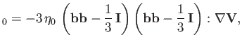
The tensor
![]()
![]() describes what is known as parallel viscosity.
This is a viscosity that controls the variation along magnetic field-lines of the
velocity component parallel to field-lines.
The parallel
viscosity coefficients,
describes what is known as parallel viscosity.
This is a viscosity that controls the variation along magnetic field-lines of the
velocity component parallel to field-lines.
The parallel
viscosity coefficients, ![]() and
and ![]() , are specified in Equations (4.112)-(4.113).
The parallel viscosity is unchanged from the unmagnetized case,
and is caused by the collision-induced random-walk diffusion of particles,
with frequency
, are specified in Equations (4.112)-(4.113).
The parallel viscosity is unchanged from the unmagnetized case,
and is caused by the collision-induced random-walk diffusion of particles,
with frequency ![]() , and step-length
, and step-length ![]() .
.
The tensors
![]()
![]() and
and
![]()
![]() describe what is known
as perpendicular viscosity. This is a viscosity
that controls the variation perpendicular to magnetic field-lines
of the velocity components perpendicular to field-lines. The perpendicular
viscosity coefficients are given by
describe what is known
as perpendicular viscosity. This is a viscosity
that controls the variation perpendicular to magnetic field-lines
of the velocity components perpendicular to field-lines. The perpendicular
viscosity coefficients are given by
 |
(4.134) | |
 |
(4.135) |
Finally, the tensors
![]()
![]() and
and
![]()
![]() describe what is known
as gyroviscosity. This is not really viscosity at all, because the
associated viscous stresses are always perpendicular to the velocity, implying that
there is no dissipation (i.e., viscous heating) associated with
this effect. The gyroviscosity coefficients are given by
describe what is known
as gyroviscosity. This is not really viscosity at all, because the
associated viscous stresses are always perpendicular to the velocity, implying that
there is no dissipation (i.e., viscous heating) associated with
this effect. The gyroviscosity coefficients are given by
 |
(4.136) | |
 |
(4.137) |