Next: Collision Times
Up: Collisions
Previous: Coulomb Logarithm
It is convenient to define
Now, from Equation (3.106),
 |
(3.127) |
Moreover,
Hence, it is easily demonstrated that
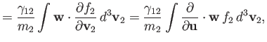
According to Equations (3.115) and (3.116),
where we have integrated the first equation by parts, making use of Equation (3.110). Thus, we deduce from Equations (3.130) and
(3.131) that
The quantities
 and
and
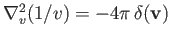
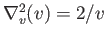
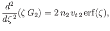
 are known as Rosenbluth potentials (Rosenbluth, MacDonald, and Judd 1957), and can easily be seen to satisfy
where
 denotes a velocity-space Laplacian operator.
The former result follows because
denotes a velocity-space Laplacian operator.
The former result follows because
 , and the
latter because
, and the
latter because
 . In particular, if
 is
isotropic in velocity space then we obtain
is
isotropic in velocity space then we obtain
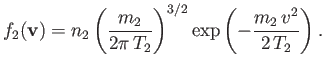
Suppose that
is a Maxwellian distribution of characteristic number density  , mean flow velocity zero, and temperature
  . In other words,
 |
(3.140) |
In this case, Equation (3.138) reduces to
 |
(3.141) |
where
 , and
, and
 . Hence, requiring
 to be finite at
  , we can integrate the
previous expression to give
, we can integrate the
previous expression to give
 |
(3.142) |
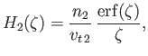
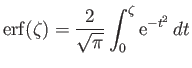
where
 |
(3.143) |
is a so-called error function (Abramowitz and Stegun 1965b). This function is such that
![$\displaystyle {\rm erf}(\zeta)= \frac{2}{\sqrt{\pi}}\left[\zeta- \frac{\zeta^{\,3}}{3}+{\cal O}\left(\zeta^{\,5}\right)\right]$](img895.png) |
(3.144) |
when
 , and
, and
![$\displaystyle {\rm erf}(\zeta)= 1- \frac{{\rm e}^{-\zeta^{\,2}}}{\sqrt{\pi}\,\zeta}\left[1+{\cal O}\left(\frac{1}{\zeta^{\,2}}\right)\right]$](img897.png) |
(3.145) |
when
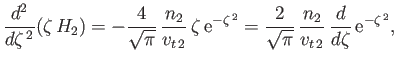
 . Equation (3.139) yields
 |
(3.146) |
which can be integrated, subject to the constraint that  be finite at
, to give
be finite at
, to give
![$\displaystyle G_2(\zeta) = \frac{n_2\,v_{t\,2}}{2\,\zeta}\left[\zeta\,\frac{d\,{\rm erf}}{d\zeta}+\left(1+2\,\zeta^{\,2}\right){\rm erf}(\zeta)\right].$](img901.png) |
(3.147) |
According to Equations (3.128), (3.129), (3.142), and (3.147),
where
Finally, it follows from Equations (3.114), (3.134), (3.135), (3.148), and (3.149) that
 |
![$\displaystyle =-\frac{\gamma_{12}\,n_2}{m_2}\left\{2\,F_1(\zeta)\,\frac{\bf v}{...
...c{{\bf v}{\bf v}}{v^2}\right]\cdot\frac{\partial f_1}{\partial{\bf v}}\right\}.$](img913.png) |
|
| |
|
(3.153) |
Suppose that
 is a Maxwellian distribution of characteristic number density
  , mean flow velocity zero, and temperature
  . In other words,
 |
(3.154) |
It follows that
 |
(3.155) |
Hence, Equations (3.113) and (3.153) yield
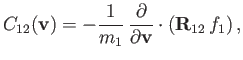 |
(3.156) |
where
 |
(3.157) |
and use has been made of the fact that
 .
The ensemble-averaged kinetic equation, Equation (3.9), can thus be written in the
form
.
The ensemble-averaged kinetic equation, Equation (3.9), can thus be written in the
form
![$\displaystyle \frac{\partial f_1}{\partial t} + \frac{\partial}{\partial {\bf r...
...artial}{\partial{\bf v}}\cdot\left[({\bf F}_1+{\bf R}_{12})\,f_1\right]={\bf0},$](img922.png) |
(3.158) |
where
 |
(3.159) |
is the ensemble-averaged Lorentz force.
In deriving Equation (3.158), we have made use of the easily proved result
 |
(3.160) |
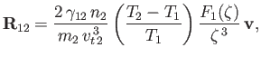
According to Equation (3.158),
collisions with particles of type  give rise to a velocity dependent effective force,
 , acting on individual particles of type
  .
As expected, this force is zero if the temperatures of the two species are equal. On the other hand, if particles of type
have a higher kinetic temperature than particles of type
(i.e., if
.
As expected, this force is zero if the temperatures of the two species are equal. On the other hand, if particles of type
have a higher kinetic temperature than particles of type
(i.e., if  ) then the collisional force acts to speed up the latter particles--in other words, the force always acts in the same direction as
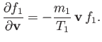
the particle's instantaneous velocity. [This follows because
) then the collisional force acts to speed up the latter particles--in other words, the force always acts in the same direction as
the particle's instantaneous velocity. [This follows because
 .] Conversely, if particles of type
have a lower kinetic temperature than particles of type
, then the collisional force acts to slow down the latter particles--in other words, the force always acts in the
opposite direction to the particle's instantaneous velocity. In both cases, the collisional force is clearly acting to equalize the kinetic temperatures.
.] Conversely, if particles of type
have a lower kinetic temperature than particles of type
, then the collisional force acts to slow down the latter particles--in other words, the force always acts in the
opposite direction to the particle's instantaneous velocity. In both cases, the collisional force is clearly acting to equalize the kinetic temperatures.
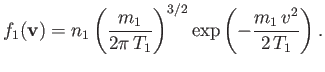
Suppose that
is a Maxwellian distribution of characteristic number density
, mean flow velocity  , and temperature
. In other words,
, and temperature
. In other words,
![$\displaystyle f_1({\bf v})=n_1\left(\frac{m_1}{2\pi\,T_2}\right)^{3/2}\exp\left[-\frac{m_1\,({\bf v}-{\bf V})^2}{2\,T_2}\right].$](img928.png) |
(3.161) |
It follows that
 |
(3.162) |
Hence, Equation (3.153) yields
![$\displaystyle {\bf A}_{12} =- \frac{\gamma_{12}\,n_2}{m_2}\left[-\frac{F_2(\zet...
...,{\bf V} + \frac{3\,F_3(\zeta)}{v^5}\,({\bf v}\cdot{\bf V})\,{\bf v}\right]f_1,$](img930.png) |
(3.163) |
which implies that
 |
(3.164) |
where
![$\displaystyle {\bf R}_{12} =- \frac{\gamma_{12}\,n_2}{m_2}\left[-\frac{F_2(\zet...
...3}\,{\bf V} + \frac{3\,F_3(\zeta)}{v^5}\,({\bf v}\cdot{\bf V})\,{\bf v}\right].$](img932.png) |
(3.165) |
As before, collisions with particles of type
give rise to a velocity dependent effective force,
,
acting on individual particles of type
.
In particular, if  is parallel to
, then
is parallel to
, then
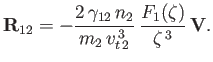 |
(3.166) |
We conclude that particles of type
moving parallel to the mean drift velocity
(of particles of type
relative to particles of type
) experience a velocity dependent force
due to collisions with particles of type
, which acts to reduce their speed. Of course, this has the effect of reducing the drift velocity.
It is easily demonstrated that
 as
as
 . Hence, Equations (3.157) and (3.166) yield
 and
and
 , respectively, in the limit
 , implying that collisions only have a relatively weak effect on high speed
particles. In fact, collisions are unable to prevent an imposed electric field from accelerating super-thermal particles (whose number is generally only a very small
fraction of the total number of particles) to relativistic speeds (Rose and Clark 1961). Such particles
are known as runaway particles.
, implying that collisions only have a relatively weak effect on high speed
particles. In fact, collisions are unable to prevent an imposed electric field from accelerating super-thermal particles (whose number is generally only a very small
fraction of the total number of particles) to relativistic speeds (Rose and Clark 1961). Such particles
are known as runaway particles.
Next: Collision Times
Up: Collisions
Previous: Coulomb Logarithm
Richard Fitzpatrick
2016-01-23


![$\displaystyle = \frac{n_2\,v_{t\,2}^{\,2}}{2\,v^3}\left[-F_2(\zeta)\,{\bf I} + 3\,F_3(\zeta)\,\frac{{\bf v}{\bf v}}{v^2}\right],$](img905.png)