Next: Exercises
Up: Charged Particle Motion
Previous: Third Adiabatic Invariant
We have seen that charged particles can be confined by a static magnetic field.
A somewhat more surprising fact is that charged
particles can also be confined by a rapidly
oscillating, inhomogeneous electromagnetic wave-field. In order to demonstrate this,
we again employ our averaging technique (Hazeltine and Waelbroeck 2004). To lowest order, a particle
executes simple harmonic motion in response to an oscillating wave-field.
However, to higher order, any weak inhomogeneity in the field causes the restoring force
at one turning point to exceed that at the other. On average, this yields a net force
that acts on the center of oscillation of the particle.
Consider a spatially inhomogeneous electromagnetic wave-field oscillating at
frequency  :
:
 |
(2.121) |
The equation of motion of a charged particle placed in this field is written
![$\displaystyle m\,\frac{d{\bf v}}{dt}= e\left[{\bf E}_0({\bf r})\,\cos(\omega\, t) +{\bf v} \times {\bf B}_0({\bf r})\,\sin(\omega\, t)\right],$](img484.png) |
(2.122) |
where
 |
(2.123) |
in accordance with Faraday's law.
In order for our averaging technique to be applicable, the electric field
 experienced by the particle must remain approximately constant
during an oscillation. Thus,
experienced by the particle must remain approximately constant
during an oscillation. Thus,
 |
(2.124) |
When this inequality is satisfied, Equation (2.123) implies that the magnetic
force experienced by the particle
is smaller than the electric force by one order in the
expansion parameter.
Let us now apply the averaging technique. We make the substitution
 in the oscillatory terms, and seek a change of variables,
such that
 and
and  are periodic functions of
  with vanishing mean. Averaging
 again yields
 to all orders. To lowest order, the momentum evolution
equation, Equation (2.122), reduces to
to all orders. To lowest order, the momentum evolution
equation, Equation (2.122), reduces to
 |
(2.127) |
Moreover, the lowest order oscillating component of
gives
 |
(2.128) |
The solutions to the previous two equations, taking into account the constraints

 , are
, are
respectively.
Here,
 represents
an oscillation average.
represents
an oscillation average.
It follows that, to lowest order, there is no motion of the center of oscillation.
To first order, the oscillation average of Equation (2.122) yields
 |
(2.131) |
which reduces to
![$\displaystyle \frac{d{\bf U}}{dt} = -\frac{e^2}{m^2\,\omega^2} \left[ ({\bf E}_...
... E}_0\times(\nabla\times{\bf E}_0)\,\langle\sin^2(\omega\,\tau)\rangle \right].$](img504.png) |
(2.132) |
The oscillation averages of the trigonometric functions are both equal to  .
Furthermore, we have
.
Furthermore, we have
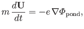
 . Thus, the equation of motion for
the center of oscillation reduces to
. Thus, the equation of motion for
the center of oscillation reduces to
 |
(2.133) |
where
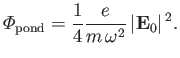 |
(2.134) |
It follows that the oscillation center experiences a force, known as the
ponderomotive force, that is proportional to the gradient
in the amplitude of the wave-field. The ponderomotive force is
independent of the sign of the charge, so both electrons and
ions can be confined in the same potential well.
The total energy of the oscillation center,
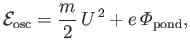 |
(2.135) |
is conserved by its equation of motion, Equation (2.133). However, it follows from Equation (2.129) that the ponderomotive
potential energy is equal to the average kinetic energy of the
oscillatory motion: that is,
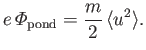 |
(2.136) |
Thus, the force on the center of oscillation originates in a transfer of
energy from the oscillatory motion to the average motion.
Most of the important applications of the ponderomotive force occur in laser
plasma physics.
For instance, a laser beam can propagate in a plasma provided that
its frequency exceeds the plasma frequency. If the beam is sufficiently
intense then plasma particles are repulsed from the center of the
beam by the ponderomotive force. The resulting variation in the plasma
density gives rise to a cylindrical well in the index of refraction
that acts as a wave-guide for the laser beam (Kruer 2003).
Next: Exercises
Up: Charged Particle Motion
Previous: Third Adiabatic Invariant
Richard Fitzpatrick
2016-01-23