Brillouin Precursor

As time progresses, the horizontal line $c\,t/x$ in Figure 12 gradually rises, and the point of stationary phase moves to ever lower frequencies. In general, however, the amplitude remains relatively small. Only when the elapsed time reaches

$$t_1 = \frac{n(0) \,x}{c}>t_0$$ (928)

is there a qualitative change. This time marks the arrival of a second precursor known as the Brillouin precursor. The reason for the qualitative change is evident from Figure 12. At $t=t_1$ , the lower region of the $c/v_g$ curve is intersected for the first time, and $\omega=0$ becomes a point of stationary phase. It follows that the oscillation frequency of the Brillouin precursor is far less than that of the Sommerfeld precursor. Moreover, it is easily demonstrated that the second derivative of $k(\omega)$ vanishes at $\omega=0$ . This means that $\phi_s''=0$ . The stationary phase result (918) gives an infinite answer in such circumstances. Of course, the amplitude of the Brillouin precursor is not infinite, but it is significantly larger than that of the Sommerfeld precursor.

In order to generalize the result (918) to deal with a stationary phase point at $\omega=0$ , it is necessary to expand $\phi(\omega)$ about this point, keeping terms up to $\omega^{\,3}$ . Thus,

$$\phi(\omega) \simeq \omega\,(t_1-t) + \frac{x}{6}\,k_0'''\,\omega^{\,3},$$ (929)

where

$$k_0'''\equiv\left(\frac{d^{\,3} k}{d\omega^{\,3}}\right)_{\omega=0} = \frac{3\,\omega_p^{\,2}} {c \,n(0)\, \omega_0^{\,4}}$$ (930)

for the simple dispersion relation (871). The amplitude (910) is therefore given approximately by

$$f(x,t) \simeq F(0) \int_{\infty}^{-\infty} \exp\left[{\rm i}\,\omega\,(t_1-t) + {\rm i}\,\frac{x}{6} \,k_0'''\, \omega^{\,3}\right]d\omega.$$ (931)

This expression reduces to

$$f(x,t) = \frac{\tau}{\sqrt{2}\,\pi^{\,2}}\sqrt{\frac{\vert t-t_1\... ...y \cos\!\left[ \frac{3}{2}\, z\left(\frac{v^{\,3}}{3} \pm v\right) \right]\,dv,$$ (932)

where

$$v = \sqrt{\frac{x\,k_0'''}{2\,\vert t-t_1\vert}}\,\,\omega,$$ (933)

and

$$z = \frac{2\sqrt{2}\, \vert t-t_1\vert^{\,3/2}}{3 \sqrt{x\, k_0'''}}.$$ (934)

The positive (negative) sign in the integrand is taken for $t<t_1$ ($t>t_1$ ).

The integral in Equation (933) is known as an Airy integral. It can be expressed in terms of Bessel functions of order $1/3$ , as follows:

$$\int_0^\infty \cos\!\left[ \frac{3}{2} \,z\left(\frac{v^{\,3}}{3} + v\right) \right]\,dv= \frac{1}{\sqrt{3}} \,K_{1/3}(z),$$ (935)

and

$$\int_0^\infty \cos\!\left[ \frac{3}{2}\, z\left(\frac{v^{\,3}}{3} - v\right) \right]\,dv= \frac{\pi}{3} \left[ J_{1/3}(z) + J_{-1/3}(z)\right].$$ (936)

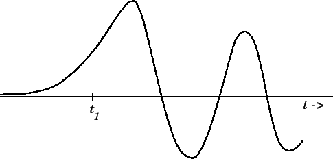
From the well-known properties of Bessel functions, the precursor can be seen to have a growing exponential character for times earlier than $t=t_1$ , and an oscillating character for $t>t_1$ . The amplitude in the neighborhood of $t=t_1$ is plotted in Figure 13.

Figure 13: A sketch of the behavior of the Brillouin precursor as a function of time.

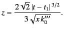
The initial oscillation period of the Brillouin precursor is crudely estimated (by setting $z\sim 1$ ) as

$${\mit\Delta} t_0 \sim (x\, k_0''')^{1/3}.$$ (937)

The amplitude of the Brillouin precursor is approximately

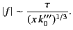$$\vert f\vert \sim \frac{\tau}{ (x \,k_0''')^{1/3}}.$$ (938)

Let us adopt the ordering

$$1/\tau \sim \omega_0 \sim \omega_p \ll \xi,$$ (939)

which corresponds to the majority of physical situations involving the propagation of electromagnetic radiation through dielectric media. It follows, from the previous results, plus the results of Section 7.11, that

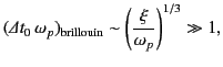$$({\mit\Delta} t_0 \,\omega_p)_{\rm brillouin} \sim \left(\frac{\xi} {\omega_p}\right)^{1/3} \gg 1,$$ (940)

and

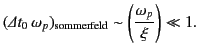$$({\mit\Delta} t_0 \,\omega_p)_{\rm sommerfeld} \sim \left(\frac{\omega_p} {\xi}\right) \ll 1.$$ (941)

Furthermore,

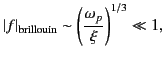$$\vert f\vert _{\rm brillouin} \sim \left(\frac{\omega_p}{\xi}\right)^{1/3} \ll 1,$$ (942)

and

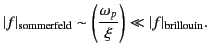$$\vert f\vert _{\rm sommerfeld} \sim \left(\frac{\omega_p}{\xi}\right) \ll \vert f\vert _{\rm brillouin}.$$ (943)

Thus, it is clear that the Sommerfeld precursor is essentially a low amplitude, high frequency signal, whereas the Brillouin precursor is a high amplitude, low frequency signal. Note that the amplitude of the Brillouin precursor, despite being significantly higher than that of the Sommerfeld precursor, is still much less than that of the incident wave.