


Next: Sommerfeld Precursor
Up: Wave Propagation in Uniform
Previous: Wave Propagation in Dispersive
It is helpful to define
 |
(871) |
Let us consider the two cases  and
and  separately.
Suppose that
. In this case, we distort the path  , used to
evaluate the integral (870), into the path
, used to
evaluate the integral (870), into the path  shown in Figure 8. This
is only a sensible thing to do if the real part of
shown in Figure 8. This
is only a sensible thing to do if the real part of
 is negative at infinity in the upper half-plane. Now, it is clear from the
dispersion relation (871) that
is negative at infinity in the upper half-plane. Now, it is clear from the
dispersion relation (871) that
 in the limit
 . Thus,
 |
(872) |
It follows that
possesses a large negative real
part along path
provided that
. Thus, Equation (870)
yields
 |
(873) |
for
. In other words, it is impossible for the wave-front
to propagate through the dispersive medium with a velocity greater than
the velocity of light in a vacuum.
Suppose that
. In this case, we distort the path
into the
lower half-plane, because
 has a negative real part at infinity in this region. In
doing this, the path becomes stuck not only at the singularity of the
denominator at
has a negative real part at infinity in this region. In
doing this, the path becomes stuck not only at the singularity of the
denominator at
 , but also at the branch
points of the expression for
, but also at the branch
points of the expression for  . After a little algebra, the dispersion
relation (871) yields
. After a little algebra, the dispersion
relation (871) yields
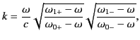 |
(874) |
where
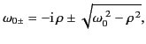 |
(875) |
and
 |
(876) |
Here,
 |
(877) |
is the plasma frequency, and
 |
(878) |
parameterizes the damping.
In order to prevent multiple roots of Equation (875), it is necessary to
place branch cuts between
 and
and
 , and also
between
, and also
between
 and
and
 . (See Figure 8.)
Figure 8:
Sketch of the integration contours used to evaluate Equation (870).
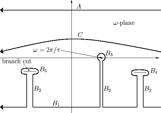 |
The path of integration  is conveniently split into the parts
 through
  . (See Figure 8.) The contribution from
is negligible, because
the exponential in Equation (870) is vanishingly small on this part of
the integration path. Likewise, the contribution from
. (See Figure 8.) The contribution from
is negligible, because
the exponential in Equation (870) is vanishingly small on this part of
the integration path. Likewise, the contribution from  is zero,
because its two sections always cancel one another. The contribution
from
is zero,
because its two sections always cancel one another. The contribution
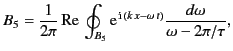
from  follows from the residue theorem:
![$\displaystyle B_3 = \frac{1}{2\pi}\, {\rm Re} \left(2\pi\,{\rm i}\,{\rm e}^{{\rm i}\,[k_\tau\, x- 2\pi\, t/\tau]}\right).$](img1827.png) |
(879) |
Here,  denotes the value of
obtained from the dispersion relation
(871) in the limit
denotes the value of
obtained from the dispersion relation
(871) in the limit
 . Thus,
![$\displaystyle B_3 = {\rm e}^{-{\rm Im}(k_\tau)\, x} \sin\left[2\pi\,\frac{t}{\tau} -{\rm Re}(k_\tau)\,x\right].$](img1830.png) |
(880) |
In general, the contributions from  and
cannot be simplified
further. For the moment, we denote them as
and
cannot be simplified
further. For the moment, we denote them as
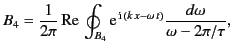 |
(881) |
and
 |
(882) |
where the paths of integration circle the appropriate branch cuts.
Altogether, we have
![$\displaystyle f(x,t) = {\rm e}^{-{\rm Im}(k_\tau)\, x} \sin\left[2\pi\,\frac{t}{\tau} -{\rm Re}(k_\tau)\,x\right]+ B_4 + B_5$](img1834.png) |
(883) |
for
.
Let us now look at the special case  . For this value of
  , we can change
the original path of integration to one at infinity in either the
upper or the lower half plane, because the integrand vanishes in each
case, through no longer exponentially, but rather as
, we can change
the original path of integration to one at infinity in either the
upper or the lower half plane, because the integrand vanishes in each
case, through no longer exponentially, but rather as
 .
We can see this from Equation (867), which can be written in the form
.
We can see this from Equation (867), which can be written in the form
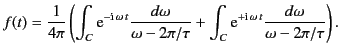 |
(884) |
Substitution of  for
for  in the second integral yields
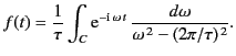 |
(885) |
Now, applying dispersion theory, we obtain from the previous equation, just as we obtained
Equation (870) from Equation (867),
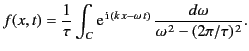 |
(886) |
Clearly, the integrand vanishes as
 in the limit that
 becomes very large. Thus, it vanishes as
for
.
Because we can calculate
becomes very large. Thus, it vanishes as
for
.
Because we can calculate  using either path
or path
,
we conclude that
using either path
or path
,
we conclude that
![$\displaystyle f(x,t) = {\rm e}^{-{\rm Im}(k_\tau)\, x} \sin\!\left[2\pi\,\frac{t}{\tau} -{\rm Re}(k_\tau)\,x\right]+ B_4 + B_5 = 0$](img1844.png) |
(887) |
for
. Thus, there is continuity in the transition from the region
to the region
.
We are now in a position to make some meaningful statements regarding the
behavior of the signal at depth  within the dispersive medium.
Prior to the time
within the dispersive medium.
Prior to the time  , there is no wave motion. In other words, even if the phase velocity
is superluminal, no electromagnetic signal can arrive earlier than one propagating
at the velocity of light in vacuum,
, there is no wave motion. In other words, even if the phase velocity
is superluminal, no electromagnetic signal can arrive earlier than one propagating
at the velocity of light in vacuum,  . The wave motion
for
. The wave motion
for  is conveniently divided into two parts:
free oscillations and
forced oscillations. The former are given by
is conveniently divided into two parts:
free oscillations and
forced oscillations. The former are given by  ,
and the latter by
,
and the latter by
![$\displaystyle {\rm e}^{-{\rm Im}(k_\tau)\, x} \sin\!\left[2\pi\,\frac{t}{\tau} ...
...\tau)\, x} \sin\!\left( \frac{2\pi}{\tau}\left[t - \frac{x}{v_p}\right]\right),$](img1848.png) |
(888) |
where
 |
(889) |
is termed the phase velocity. The forced oscillations have the
same sine wave characteristics and oscillation frequency as the incident
wave.
However, the wave amplitude is diminished by the damping coefficient, although,
as we have seen,
this is generally a negligible effect unless the frequency of the incident
wave closely matches one of the resonant frequencies of the dispersive
medium. The phase velocity  determines the velocity at which
a point of constant phase (e.g., a peak or trough) of the forced oscillation signal
propagates into the medium. However, the phase
velocity has no effect on the velocity
at which the forced oscillation wave-front propagates
into the medium. This latter velocity is equivalent to the velocity
of light in vacuum,
. The phase velocity
can be either greater or less than
, in which case peaks and troughs either catch up with or fall further
behind the wave-front. Of course, peaks can never overtake the wave-front.
determines the velocity at which
a point of constant phase (e.g., a peak or trough) of the forced oscillation signal
propagates into the medium. However, the phase
velocity has no effect on the velocity
at which the forced oscillation wave-front propagates
into the medium. This latter velocity is equivalent to the velocity
of light in vacuum,
. The phase velocity
can be either greater or less than
, in which case peaks and troughs either catch up with or fall further
behind the wave-front. Of course, peaks can never overtake the wave-front.
It is clear from Equations (876), (877), (882), and (883) that the free
oscillations oscillate with real frequencies that lie somewhere between
the resonant frequency,  , and the plasma frequency,
  .
Furthermore, the free oscillations are damped in time
like
.
Furthermore, the free oscillations are damped in time
like
 . The free oscillations, like the
forced oscillations, begin at time
. At
, the free
and forced oscillations exactly cancel one another [see Equation (888)]. As
. The free oscillations, like the
forced oscillations, begin at time
. At
, the free
and forced oscillations exactly cancel one another [see Equation (888)]. As
 increases, both the free and
forced oscillations set in, but the former rapidly damp away, leaving only
the forced oscillations. Thus, the free oscillations can be
regarded as
some sort of transient response of the medium to the incident
wave, whereas the forced oscillations determine the time asymptotic
response. The real frequency of the forced oscillations is that imposed
externally by the incident wave, whereas the real frequency of the free
oscillations is determined by the nature of the dispersive medium, quite
independently of the frequency of the incident wave.
increases, both the free and
forced oscillations set in, but the former rapidly damp away, leaving only
the forced oscillations. Thus, the free oscillations can be
regarded as
some sort of transient response of the medium to the incident
wave, whereas the forced oscillations determine the time asymptotic
response. The real frequency of the forced oscillations is that imposed
externally by the incident wave, whereas the real frequency of the free
oscillations is determined by the nature of the dispersive medium, quite
independently of the frequency of the incident wave.
One slightly surprising result of the previous analysis is the prediction that
the signal wave-front propagates into the dispersive medium
at the velocity of light in vacuum, irrespective of the
dispersive properties of the medium. Actually, this is a fairly
obvious result. As is well described by Feynman in his famous
Lectures on Physics, when an electromagnetic wave propagates through
a dispersive medium, the electrons and ions that make up
that medium oscillate in
sympathy with the incident wave, and, in doing so, emit radiation. The radiation from the electrons and ions, as well as the incident radiation,
travels at the velocity
. However, when these two radiation signals
are superposed, the net effect is as if the incident signal propagates through
the dispersive medium at a phase velocity that is different
from
. Consider the wave-front of the incident signal, which
clearly propagates
into the medium with the velocity
. Prior to the arrival of this
wave-front, the electrons and ions are at rest, because no information regarding the
arrival of the incident wave at the surface of the medium can propagate faster than
.
After the arrival of the
wave-front, the electrons and ions are set into motion, and
emit radiation which affects the apparent phase velocity
of radiation that arrives somewhat later. But this radiation
certainly cannot affect the propagation velocity of the wave-front
itself, which has already passed by the time the electrons and ions
are set into motion (because of their finite inertia).
Next: Sommerfeld Precursor
Up: Wave Propagation in Uniform
Previous: Wave Propagation in Dispersive
Richard Fitzpatrick
2014-06-27