Next: Wave Propagation in Uniform
Up: Magnetostatics in Magnetic Media
Previous: Magnetic Energy
- Given that the bound charge density associated with a polarization field
 is
is
 , use charge conservation to deduce that the current density due to bound
charges is
, use charge conservation to deduce that the current density due to bound
charges is
- Given that
 in the absence of true currents, and
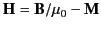 , demonstrate that
the current density due to magnetization currents is
, demonstrate that
the current density due to magnetization currents is
- A cylindrical hole of radius
 is bored parallel to the axis of a cylindrical conductor of
radius
is bored parallel to the axis of a cylindrical conductor of
radius  which carries a uniformly distributed current of density
  running parallel to its axis.
The distance between the center of the conductor and the center of the hole is
running parallel to its axis.
The distance between the center of the conductor and the center of the hole is  . Find the
  field in the hole.
- A sphere of radius
carries a uniform surface charge density
 . The sphere is rotated about
a diameter with constant angular velocity
. The sphere is rotated about
a diameter with constant angular velocity  . Find the vector potential and the
field
both inside and outside the sphere.
. Find the vector potential and the
field
both inside and outside the sphere.
- Find the
and
 fields inside and outside a spherical shell of inner radius
and
outer radius
fields inside and outside a spherical shell of inner radius
and
outer radius  which is magnetized permanently to a constant magnetization
  .
.
- A long hollow, right cylinder of inner radius
and outer radius
, and of relative
permeability
 , is placed in a region of initially uniform magnetic flux density
at
right-angles to the field. Find the flux density at all points in space. Neglect end effects.
, is placed in a region of initially uniform magnetic flux density
at
right-angles to the field. Find the flux density at all points in space. Neglect end effects.
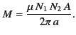
- A transformer consists of a thin uniform ring of ferromagnetic material of radius
,
cross-sectional area
 , and magnetic permeability
. The primary
circuit is wrapped
, and magnetic permeability
. The primary
circuit is wrapped  times around one side of the ring, and the
secondary
times around one side of the ring, and the
secondary  times around the other side. Show that the mutual inductance
between the two circuits is
times around the other side. Show that the mutual inductance
between the two circuits is
Suppose that a thin gap of thickness  is cut in a part of the ring in which there
are no windings. What is the new mutual inductance of the two circuits?
Suppose that the gap is filled with ferromagnetic material of
permeability
is cut in a part of the ring in which there
are no windings. What is the new mutual inductance of the two circuits?
Suppose that the gap is filled with ferromagnetic material of
permeability  . What, now, is the mutual inductance of the circuits?
You may neglect flux-leakage (i.e., you may assume that magnetic field-lines do not leak out of the transformer core into the surrounding vacuum, except in the gap).
. What, now, is the mutual inductance of the circuits?
You may neglect flux-leakage (i.e., you may assume that magnetic field-lines do not leak out of the transformer core into the surrounding vacuum, except in the gap).
Next: Wave Propagation in Uniform
Up: Magnetostatics in Magnetic Media
Previous: Magnetic Energy
Richard Fitzpatrick
2014-06-27