Next: Radiation from Linear Centre-Fed
Up: Multipole Expansion
Previous: Solution of Inhomogeneous Helmholtz
Let us now examine the connection between multipole fields and
their sources. Suppose that there exist localized distributions
of
electric change,
 , true current,
 ,
and magnetization,
,
and magnetization,
 . We assume that any time
dependence can be analyzed into its Fourier components, and we
therefore only consider
harmonically varying sources,
. We assume that any time
dependence can be analyzed into its Fourier components, and we
therefore only consider
harmonically varying sources,
 ,
,
 ,
and
,
and
 ,
where it is understood that we take the real parts of complex quantities.
,
where it is understood that we take the real parts of complex quantities.
Maxwell's equations can be written
 |
 |
(1516) |
 |
 |
(1517) |
 |
 |
(1518) |
 |
 |
(1519) |
whereas the charge continuity equation takes the form
 |
(1520) |
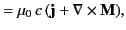
It is convenient to deal only with divergence-free fields. Thus, we use as our
field variables,  and
and
 |
(1521) |
In the region external to the sources,  reduces to
  .
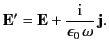
When expressed in terms of these fields, Maxwell's equations become
.
When expressed in terms of these fields, Maxwell's equations become
 |
|
(1522) |
|
|
(1523) |
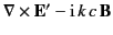 |
 |
(1524) |
 |
 |
(1525) |
The curl equations can be combined to give two inhomogeneous Helmholtz
wave equations:
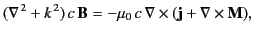 |
(1526) |
and
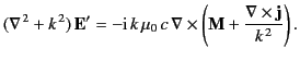 |
(1527) |
These equations, together with
 , and
, and
 , as well as the curl equations giving
in terms of
, and vice versa, are the generalizations of
Equations (1455)-(1460) when sources are present.
, as well as the curl equations giving
in terms of
, and vice versa, are the generalizations of
Equations (1455)-(1460) when sources are present.
Because the multipole coefficients in Equations (1479)-(1480) are determined, via
Equations (1483)-(1484), from the scalars
 and
and
 , it is sufficient to consider wave equations
for these quantities, rather than the vector fields
and
. From Equations (1462), (1528), (1529), and the identity
, it is sufficient to consider wave equations
for these quantities, rather than the vector fields
and
. From Equations (1462), (1528), (1529), and the identity
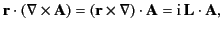 |
(1528) |
which holds for any vector field  , we obtain the inhomogeneous
wave equations
, we obtain the inhomogeneous
wave equations
Now, the Green's function for the inhomogeneous Helmholtz equation, subject to the boundary condition of outgoing waves
at infinity, is given by Equation (1509). It follows that
Equations (1531)-(1532) can be inverted to give
In order to evaluate the multipole coefficients by means of
Equations (1483)-(1484), we first observe that the requirement of outgoing waves at
infinity implies that
 in Equation (1467). Thus, in Equations (1479)-(1480), we choose
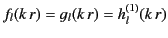 as the radial eigenfunctions
of
and
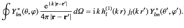
in the source-free region. Next, let us consider the expansion (1517) of the Green's function for the inhomogeneous Helmholtz equation. We assume that the point
as the radial eigenfunctions
of
and
in the source-free region. Next, let us consider the expansion (1517) of the Green's function for the inhomogeneous Helmholtz equation. We assume that the point  lies
outside some spherical shell that completely encloses the sources. It follows
that
lies
outside some spherical shell that completely encloses the sources. It follows
that  and
and  in all of the integrations. Making use
of the orthogonality property of the spherical harmonics, it follows
from Equation (1517) that
in all of the integrations. Making use
of the orthogonality property of the spherical harmonics, it follows
from Equation (1517) that
 |
(1533) |
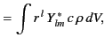
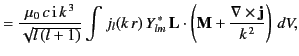
Finally, Equations (1483)-(1484), and (1533)-(1535) yield
The previous two equations allow us to calculate the strengths of the various multipole
fields, external to the source region, in terms of integrals over the source
densities,  and
and  . These equations can be transformed into more
useful forms by means of the following arguments. The results
. These equations can be transformed into more
useful forms by means of the following arguments. The results
follow from the definition of  [see (1438)], and simple vector identities.
Substituting into Equation (1536), we obtain
[see (1438)], and simple vector identities.
Substituting into Equation (1536), we obtain
![$\displaystyle a_E(l,m) = - \frac{\mu_0\, c\,\,k^{\,3}}{\sqrt{l\,(l+1)}} \int j_...
...}} -{\rm i}\,\frac{c}{k\,r} \frac{\partial(r^{\,2} \rho)}{\partial r}\right]dV,$](img3227.png) |
(1538) |
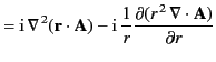
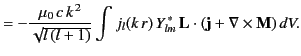
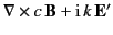
where use has been made of Equation (1522). Use of Green's theorem on the
second term in square brackets allows us to replace
 by
by  (because we can neglect
surface terms, and
(because we can neglect
surface terms, and
 is a solution of the Helmholtz
equation). A radial integration by parts on the third term (again
neglecting surface terms) cause the radial derivate to operate on
the spherical Bessel function. The resulting expression for the electric multipole coefficient is
is a solution of the Helmholtz
equation). A radial integration by parts on the third term (again
neglecting surface terms) cause the radial derivate to operate on
the spherical Bessel function. The resulting expression for the electric multipole coefficient is
![$\displaystyle a_E(l,m) = \frac{\mu_0\, c\,k^{\,2}}{{\rm i}\,\sqrt{l\,(l+1)}} \i...
...,j_l(k\,r)-{\rm i}\,k\,\nabla\cdot({\bf r}\times{\bf M})\,j_l(k\,r)\right]\,dV.$](img3230.png) |
(1539) |
Similarly, Equation (1537) leads to the following
expression for the magnetic multipole coefficient:
![$\displaystyle a_M(l,m) = \frac{\mu_0\, c\,k^{\,2}}{{\rm i}\,\sqrt{l\,(l+1)}} \i...
...\frac{d [r\,j_l(k\,r)]}{d r}-k^2\,({\bf r}\cdot{\bf M})\,j_l(k\,r) \right]\,dV.$](img3231.png) |
(1540) |
Both of the previous results are exact, and are valid for arbitrary wavelength
and source size.
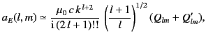
In the limit in which the source dimensions are small compared
to a wavelength (i.e.,  ), the above expressions for the
multipole coefficients can be considerably simplified. Using the
asymptotic form (1428), and retaining only lowest powers in
), the above expressions for the
multipole coefficients can be considerably simplified. Using the
asymptotic form (1428), and retaining only lowest powers in  for
terms involving
for
terms involving  ,
, and
, we obtain the
approximate electric multipole coefficient
,
, and
, we obtain the
approximate electric multipole coefficient
 |
(1541) |
where the multipole moments are
The moment  has the same form as a conventional electrostatic
multipole moment. The moment
has the same form as a conventional electrostatic
multipole moment. The moment  is an induced electric multipole
moment due to the magnetization. The latter moment is generally a factor
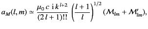
smaller than the former. For the magnetic multipole
coefficient
is an induced electric multipole
moment due to the magnetization. The latter moment is generally a factor
smaller than the former. For the magnetic multipole
coefficient  , the corresponding long wavelength approximation
is
, the corresponding long wavelength approximation
is
 |
(1544) |
where the magnetic multipole moments are
Note that for a system with intrinsic magnetization, the magnetic
moments
 and
and
 are generally of
the same order of magnitude.
We conclude that, in the long wavelength limit, the electric multipole fields are
determined by the charge density,
, whereas the magnetic multipole
fields are determined by the magnetic moment densities,
are generally of
the same order of magnitude.
We conclude that, in the long wavelength limit, the electric multipole fields are
determined by the charge density,
, whereas the magnetic multipole
fields are determined by the magnetic moment densities,
 and
.
and
.
Next: Radiation from Linear Centre-Fed
Up: Multipole Expansion
Previous: Solution of Inhomogeneous Helmholtz
Richard Fitzpatrick
2014-06-27
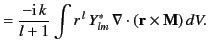
![$\displaystyle =\frac{{\rm i}\,\mu_0\, c}{4\pi} \int\frac{{\rm e}^{\,{\rm i}\,k\...
...\bf L}'\cdot\left[{\bf j}({\bf r}') +\nabla'\times {\bf M}({\bf r}')\right]dV',$](img3211.png)
![$\displaystyle = -\frac{k\,\mu_0 \, c}{4\pi}\int \frac{{\rm e}^{\,{\rm i}\,k\,\v...
...t\left[{\bf M}({\bf r}')+\frac{\nabla'\times {\bf j}({\bf r}')}{k^2}\right]dV'.$](img3213.png)