Cavities with Rectangular Boundaries

Consider a rectangular vacuum region totally enclosed by conducting walls. In this case, all of the field components satisfy the wave equation

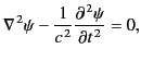$$\nabla^{\,2}\psi - \frac{1}{c^{\,2}}\frac{\partial^{\,2}\psi}{\partial t^{\,2}}=0,$$ (1307)

where $\psi$ represents any component of ${\bf E}$ or ${\bf H}$ . The boundary conditions (1302)-(1305) require that the electric field at the boundary be normal to the conducting walls, whereas the magnetic field be tangential. If $a$ , $b$ , and $c$ are the dimensions of the cavity, in the $x$ , $y$ , and $z$ directions, respectively, then it is readily verified that the electric field components are

$$E_x(x,y,z,t) = E_1\, \cos(k_1 \,x)\sin(k_2 \,y) \sin(k_3\, z)\, {\rm e}^{-{\rm i}\,\omega\, t},$$ (1308)

$$E_y(x,y,z,t) = E_2\, \sin(k_1 \,x)\cos(k_2\, y) \sin(k_3 \,z)\, {\rm e}^{-{\rm i}\,\omega \,t},$$ (1309)

$$E_z(x,y,z,t) = E_3 \,\sin(k_1 \,x)\sin(k_2 \,y) \cos(k_3 \,z)\, {\rm e}^{-{\rm i}\,\omega\, t},$$ (1310)

where

$$k_1 = \frac{l\,\pi}{a},$$ (1311)

$$k_2 = \frac{m\,\pi}{b},$$ (1312)

$$k_3 = \frac{n\,\pi}{c}.$$ (1313)

Here, $l$ , $m$ , $n$ are non-negative integers. The allowed frequencies are given by

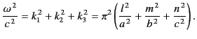$$\frac{\omega^{\,2}}{c^{\,2}} = k_1^{\,2}+k_2^{\,2}+k_3^{\,2}=\pi^... ...c{l^{\,2}}{a^{\,2}} + \frac{m^{\,2}}{b^{\,2}} + \frac{n^{\,2}}{c^{\,2}}\right).$$ (1314)

It is clear from Equations (1310)-(1312) that at least two of the integers $l$ , $m$ , $n$ must be different from zero in order to have non-vanishing fields. The magnetic fields, obtained by solving $\nabla\times{\bf E}={\rm i}\,\omega\,{\bf B}$ , automatically satisfy the appropriate boundary conditions, and are in phase quadrature with the corresponding electric fields. Thus, the sum of the total electric and magnetic energies within the cavity is constant, although the two terms oscillate separately.

The amplitudes of the electric field components are not independent, but are related by the divergence condition $\nabla \cdot {\bf E} = 0$ , which yields

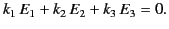$$k_1\,E_1 + k_2 \,E_2 + k_3\, E_3 = 0.$$ (1315)

There are, in general, two linearly independent vectors ${\bf E}$ that satisfy this condition, corresponding to two different polarizations. (The exception is when one of the integers $l$ , $m$ , $n$ is zero, in which case ${\bf E}$ is fixed in direction.) Each electric field vector is accompanied by a perpendicular magnetic field vector. The fields corresponding to a given set of integers $l$ , $m$ , and $n$ constitute a particular mode of oscillation of the cavity. It is evident from standard Fourier theory that the different modes are orthogonal (i.e., they are normal modes), and that they form a complete set. In other words, any general electric and magnetic fields that satisfy the boundary conditions (1302)-(1305) can be unambiguously decomposed into some linear combination of all of the various possible normal modes of the cavity. Because each normal mode oscillates at a specific frequency, it is clear that if we are given the electric and magnetic fields inside the cavity at time $t=0$ then the subsequent behavior of the fields is uniquely determined for all time.

The conducting walls gradually absorb energy from the cavity, due to their finite resistivity, at a rate that can easily be calculated. For finite $\sigma$ , the small tangential component of ${\bf E}$ at the walls can be estimated using Equation (1306):

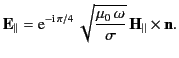$${\bf E}_\parallel = {\rm e}^{-{\rm i}\,\pi/4}\, \sqrt{\frac{\mu_0\,\omega}{\sigma}}\, {\bf H}_\parallel \times{\bf n}.$$ (1316)

Now, the tangential component of ${\bf H}$ at the walls is slightly different from that given by the ideal solution. However, this is a small effect, and can be neglected to leading order in $\sigma^{\,-1}$ . The time averaged energy flux into the walls is then given by

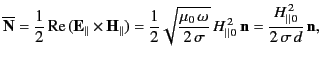$$\overline{\bf N} = \frac{1}{2} \, {\rm Re}\,({\bf E}_\parallel\ti... ... \,0}^{\,2}\,{\bf n} = \frac{H_{\parallel \,0}^{\,2}}{2\,\sigma\, d}\, {\bf n},$$ (1317)

where $H_{\parallel\, 0}$ is the peak value of the tangential magnetic field at the walls that is predicted by the ideal solution. According to the boundary condition (1305), $H_{\parallel\, 0}$ is equal to the peak value of the surface current density $K_0$ . It is helpful to define a surface resistance,

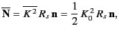$$\overline{\bf N} = \overline{K^{\,2}} \,R_s\,{\bf n}= \frac{1}{2}\,K_0^{\,2}\,R_s\,{\bf n},$$ (1318)

where

$$R_s = \frac{1}{\sigma\, d}.$$ (1319)

This approach makes it clear that the dissipation of energy in a resonant cavity is due to ohmic heating in a thin layer, whose thickness is of order the skin depth, covering the surface of the conducting walls.