Next: Radiation and Scattering
Up: Wave Propagation in Inhomogeneous
Previous: Jeffries Connection Formula
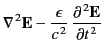
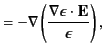
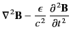
- Consider an electromagnetic wave propagating through a
nonuniform dielectric medium whose dielectric constant
 is a
function of
is a
function of  . Demonstrate that the associated
wave equations take the form
. Demonstrate that the associated
wave equations take the form
- Suppose that a light-ray is incident on the front (air/glass) interface of a uniform pane
of glass of refractive index
 at the Brewster angle. Demonstrate that the refracted ray
is also incident on the rear (glass/air) interface of the pane at the Brewster
angle.
at the Brewster angle. Demonstrate that the refracted ray
is also incident on the rear (glass/air) interface of the pane at the Brewster
angle.
- Consider an electromagnetic wave obliquely incident on a plane
boundary between two transparent magnetic media of permeabilities
 and
and  . Find the coefficients of reflection and transmission
as functions of the angle of incidence for the wave polarizations in
which all electric fields are parallel to the boundary and all magnetic
fields are parallel to the boundary. Is there a Brewster angle? If so, what is it?
Is it possible to obtain total reflection? If so, what is the critical angle of
incidence required to obtain total reflection?
. Find the coefficients of reflection and transmission
as functions of the angle of incidence for the wave polarizations in
which all electric fields are parallel to the boundary and all magnetic
fields are parallel to the boundary. Is there a Brewster angle? If so, what is it?
Is it possible to obtain total reflection? If so, what is the critical angle of
incidence required to obtain total reflection?
- A medium is such that the product of the phase and group
velocities of electromagnetic waves is equal to
 at all wave
frequencies. Demonstrate that the dispersion relation for
electromagnetic waves takes the form
at all wave
frequencies. Demonstrate that the dispersion relation for
electromagnetic waves takes the form
where  is a constant.
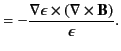
- Demonstrate that if the equivalent height of reflection in the ionosphere varies with the angular frequency of the wave as
where  ,
,  , and
are positive constants, then
, and
are positive constants, then
 for
for  , and
, and
for  . Here,
 is a Gamma function.
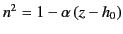
- Suppose that the refractive index,
 , of the ionosphere is given by
 for
,
and
for
,
and  for
, where
for
, where  and
are positive constants, and the Earth's magnetic field and curvature are both neglected.
Here,
and
are positive constants, and the Earth's magnetic field and curvature are both neglected.
Here,  measures altitude above the Earth's surface.
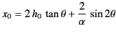
- A point transmitter sends up a wave packet at an angle
 to the vertical. Show that the packet returns to Earth a
distance
to the vertical. Show that the packet returns to Earth a
distance
from the transmitter. Demonstrate that if
 then for some values of
  the previous equation is satisfied
by three different values of
. In other words, wave packets can travel from the transmitter to the receiver via one of
three different paths. Show that the critical case
the previous equation is satisfied
by three different values of
. In other words, wave packets can travel from the transmitter to the receiver via one of
three different paths. Show that the critical case
 corresponds to
 and
and
 .
.
- A point
radio transmitter emits a pulse of radio waves uniformly in all directions. Show that the pulse first returns to the Earth a
distance
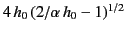 from the transmitter, provided that
 .
.
Next: Radiation and Scattering
Up: Wave Propagation in Inhomogeneous
Previous: Jeffries Connection Formula
Richard Fitzpatrick
2014-06-27
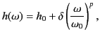
![$\displaystyle \omega_p(z) =\left[\frac{\pi\,{\mit\Gamma}(1+p)}{{\mit\Gamma}(1/2...
...2+p/2)}\right]^{1/p} \frac{\omega_0}{2}\left(\frac{z-h_0}{\delta}\right)^{1/p}
$](img2585.png)